Population coding of time-varying sounds in the non-lemniscal Inferior Colliculus

Abstract

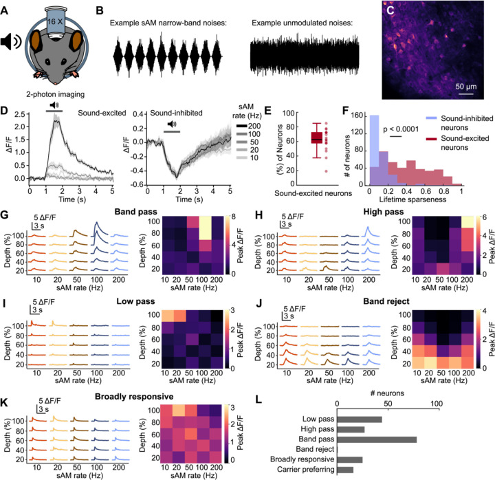
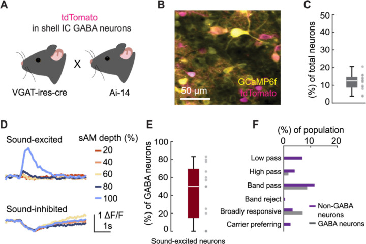
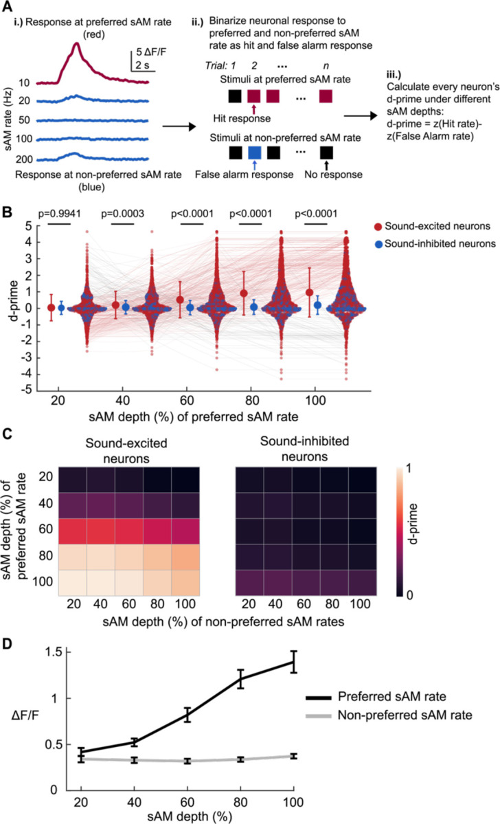
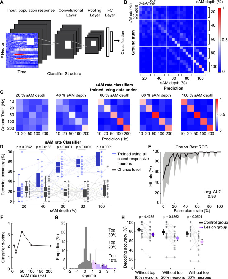
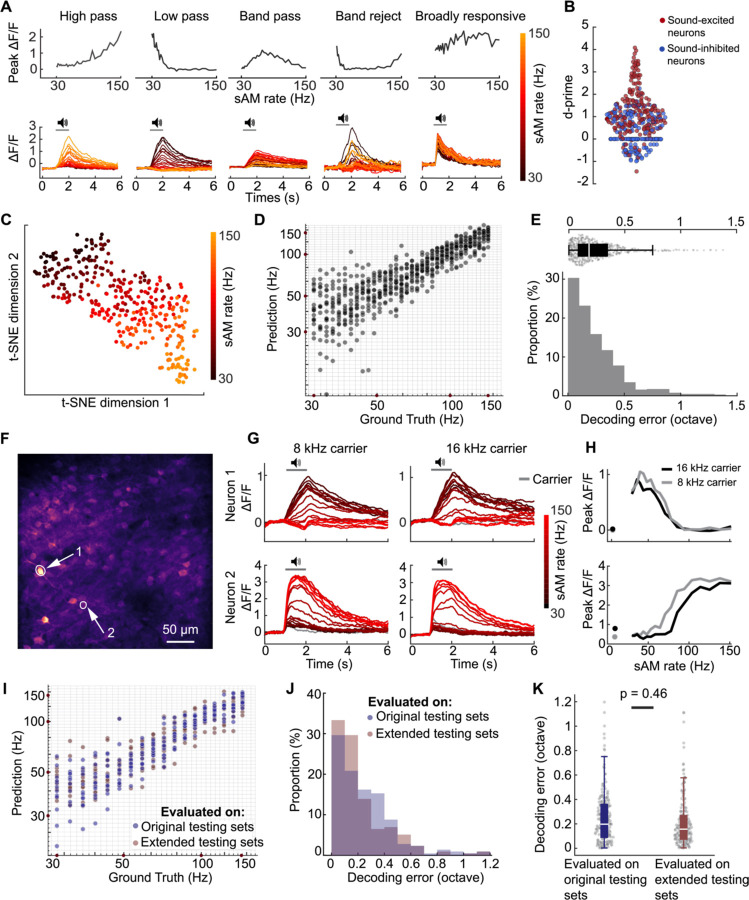
The inferior colliculus (IC) of the midbrain is important for complex sound processing, such as discriminating conspecific vocalizations and human speech. The IC's non-lemniscal, dorsal "shell" region is likely important for this process, as neurons in these layers project to higher-order thalamic nuclei that subsequently funnel acoustic signals to the amygdala and non-primary auditory cortices; forebrain circuits important for vocalization coding in a variety of mammals, including humans. However, the extent to which shell IC neurons transmit acoustic features necessary to discern vocalizations is less clear, owing to the technical difficulty of recording from neurons in the IC's superficial layers via traditional approaches. Here we use 2-photon Ca²⁺ imaging in mice of either sex to test how shell IC neuron populations encode the rate and depth of amplitude modulation, important sound cues for speech perception. Most shell IC neurons were broadly tuned, with a low neurometric discrimination of amplitude modulation rate; only a subset were highly selective to specific modulation rates. Nevertheless, neural network classifier trained on fluorescence data from shell IC neuron populations accurately classified amplitude modulation rate, and decoding accuracy was only marginally reduced when highly tuned neurons were omitted from training data. Rather, classifier accuracy increased monotonically with the modulation depth of the training data, such that classifiers trained on full-depth modulated sounds had median decoding errors of ~0.2 octaves. Thus, shell IC neurons may transmit time-varying signals via a population code, with perhaps limited reliance on the discriminative capacity of any individual neuron.

Figure 1

Responses of mouse shell IC neurons to sAM and unmodulated narrow-band noises. A. Experimental setup of sound presentation and 2-photon imaging of head-fixed, awake mice. B. Left, an example of presented sAM narrow-band noises (100% sAM depth and 10 Hz sAM rate). Right, an example of presented unmodulated noises. C. Example imaging FOV. D. Example responses of sound-excited (left), and sound-inhibited (right) neurons to fully modulated sAM sounds. Data are mean ± SEM. E. Proportion of sound-excited neurons in each imaging session. F. Distribution of lifetime sparseness of sound-excited and sound-inhibited neurons. A neuron is maximally selective to sAM stimuli if its sparseness is 1 and is totally unselective if the sparseness is 0. Mann-Whitney U test. G-K. Example of trial-averaged neuronal responses (left) and peak ΔF/F (right) of band pass (G), high pass (H), low pass (I), and band reject (J), broadly responsive (K) neurons under different sAM sounds. L. Distribution of the number of tuning characteristics of shell IC neurons.

Figure 2

sAM tuning of shell IC GABAergic and non-GABAergic neurons. A. tdTomato was expressed in GABAergic neurons in transgenic VGAT-ires-cre x Ai14 mice. B. Example imaging FOV. C. Proportion of GABAergic neurons in each imaging session. D. Examples of sound-excited and sound-inhibited responses of GABAergic neurons to sounds with 100 Hz sAM rate and different sAM depths. E. Proportion of sound-excited GABAergic neurons in each imaging session. F. Distribution of tuning characteristics of non-GABAergic and GABAergic neurons.

Figure 3

Neurometric sensitivity of individual shell IC neurons. A. Schematic of neurometric sensitivity index (d-prime) analysis. Preferred sAM rate is determined by the peak fluorescence response at different sAM rates (i). We binarize a neuron’s response as a hit if the mean neuronal response at its preferred sAM rate exceeds three times the standard deviation of the baseline fluctuation on a single trial. Similarly, we count a false alarm response if a neuron’s average response at its non-preferred sAM rate exceeds three times the standard deviation of the baseline fluctuation (ii). The d-prime was then calculated for each neuron for all pairs of sAM depths for preferred and non-preferred sAM rates (iii). B. Distribution of d-prime at varying sAM depths for the preferred sAM rate. Each line indicates a neuron displaying an increasing (pink) or decreasing (gray) trend across sAM depths for the preferred sAM rate (See Methods). Data are mean with ± std. Two-way ANOVA. Šídák’s multiple comparison between d-primes of sound-excited and sound-inhibited neurons. C. Left, averaged d-prime of sound-excited neurons. Right, averaged d-prime of sound-inhibited neurons. D. Trial-averaged fluorescence response to preferred and non-preferred sAM rate. Data are mean with ± SEM.

Figure 4

Decoding sAM features using shell IC neural population activity. A. Structure of the CNN classifier. A CNN classifier fed with Ca²⁺ signal time series was trained to classify sAM features. B. Normalized confusion matrix of sAM depth and -rate joint combination classification averaged across imaging sessions. C. Normalized confusion matrix of sAM rate classification under a given sAM depth averaged across imaging sessions. D. Decoding accuracy of the sAM rate classifier under a given depth and the corresponding chance level. Two-way repeated-measures ANOVA. Šídák’s multiple comparison between the chance level accuracy and decoding accuracy trained using all neurons. E. One-vs-rest ROC of sAM rate classification under 100% sAM depth. Data are mean with ± std. F. d-prime of sAM rate classifier under 100% sAM depth. G. Individual neuron d-prime distribution (under 100 % sAM depth), with the corresponding highly sensitive neurons falling within top deciles (10 %, 20 %, 30 % of d-prime). H. Decoding accuracy of the sAM rate classifier under 100% sAM depth, trained while excluding the top deciles (10%, 20%, 30%) of neurons, selected based on their d-prime profiles in the left panel. To rectify the effect of the number of neurons on the decoding performance of the classifier, decoding accuracy of the classifier trained with a balanced number of randomly chosen neurons was visualized as control. Data are mean with ± SEM and gray dots represent predictions from each imaging session. Two-way ANOVA. Šídák’s multiple comparison between the decoding accuracy trained without highly tuned neurons and the control.

Figure 5

Decoding sAM rate using sound-excited and sound-inhibited neurons. A. Decoding accuracy of sAM rate classifier trained using sound-inhibited neurons and corresponding chance level. Two-way repeated-measures ANOVA. Šídák’s multiple comparison between decoding accuracy trained using sound-inhibited and chance B. Decoding accuracy of sAM rate classifier trained using sound-excited neurons and corresponding chance level. To ensure an equal number of sound-excited and sound-inhibited neurons, we randomly selected a subset of sound-excited neurons from each imaging session. Two-way repeated-measures ANOVA. Šídák’s multiple comparison between decoding accuracy trained using balanced sound-excited and chance. C. Decoding accuracy of sAM rate classifier trained using all sound-responsive, sound-excited, and sound-inhibited neurons under 100 % sAM depth. Kruskal-Wallis test. Dunn’s multiple comparison between decoding accuracies trained under different conditions.

Figure 6

Decoding sAM depth. A. Decoding accuracy of the sAM depth classifier under a given rate and its corresponding chance level. Two-way repeated-measures ANOVA. Šídák’s multiple comparison between decoding accuracy trained using all neurons and the chance. B. Normalized confusion matrix of sAM depth classification under a given rate averaged across imaging sessions.

Figure 7

Representation of different sAM depths in the shell IC. A. For sAM rate classification, the decoder was trained using input data from a specific sAM depth. After training was complete, the decoder was evaluated on both original testing sets held back from training and extended testing sets (all datasets from other sAM depths). B. Evaluation of the sAM rate classifier on extended testing sets (black) and held-back testing sets (red). The curve was fitted using a gaussian model. Friedman test for each sub-panel. Dunn’s multiple comparison between decoding accuracies tested on held-back and extended testing sets. C. Pattern correlation of each pair of sAM depths. Left, Correlation of the trial-averaged neural population vector across two different sAM depths or -rates on a per-frame basis. Data are mean ± SEM Right, averaged correlation data during sound presentation. D. Two-dimensional t-SNE map of shell IC neural population activity. Left, t-SNE map of neural population activity during baseline. Right, t-SNE map of neural population activity during sound presentation. E. t-SNE map of neural population data with a single sAM depth only. Each dot represents a single trial neural population activity.

Figure 8

Binary classification of sAM and unmodulated sounds. A. Binary classification paradigm: A CNN decoder was trained to classify sAM (with different sAM depths and -rates) and unmodulated noise. B. Decoding accuracy of binary classification of sAM sounds and unmodulated noise and corresponding chance level. C. Logistic curve fitting of the binary classification performance. Dashed lines, both horizontal and vertical, denotes the position of the half maximum on the fitted curve. D. Pattern correlation between sAM sounds with different sAM depths and unmodulated sounds. For B and D, data are mean ± SEM.

Figure 9

Neuronal responses to narrowly spaced sAM rates in the shell IC. A. Examples of modulation transfer functions to fully modulated sAM sounds with 30–150 Hz sAM rates. Top: peak response of example neurons at varying sAM rates and 100% sAM depth. Bottom: trial-averaged fluorescence traces of example neurons. B. Distribution of d-prime of shell IC neurons. C. t-SNE map of shell IC population responses to narrowly spaced sAM rates. Each dot represents neural population activity in a single trial. D. Regression performance of CNN decoder using population fluorescence data of shell IC neurons with narrowly spaced sAM rates and 100% sAM depth. Each dot is the prediction of a single trial in testing sets. The coordinates are plotted on a logarithmic scale of base 10. E. Distribution of decoding errors in octaves. F. Example imaging FOV. G-H. trial-averaged responses (G) and peak of response (H) of two example neurons to sAM sounds with 16kHz and 8kHZ center frequencies for the noise carrier. I. sAM rate decoding performance: sAM rate decoder was trained using data from sAM sounds with central frequency of either 8 kHz or 16 kHz for the noise carrier. After training, the decoder was evaluated on both original held-back testing sets with the same center frequency as in the training set, and extended testing sets with a different central frequency of the carrier. J-K. Distribution of decoding error in octave. Wilcoxon signed-rank test.

References

1. Ayala YA, Udeh A, Dutta K, Bishop D, Malmierca MS, Oliver DL (2015) Differences in the strength of cortical and brainstem inputs to SSA and non-SSA neurons in the inferior colliculus. Sci Rep 5:10383. - PMC - PubMed
1. Aitkin L, Tran L, Syka J (1994) The responses of neurons in subdivisions of the inferior colliculus of cats to tonal, noise and vocal stimuli. Exp Brain Res 98:53–64. - PubMed
1. Aitkin LM, Webster WR, Veale JL, Crosby DC (1975) Inferior colliculus. I. Comparison of response properties of neurons in central, pericentral, and external nuclei of adult cat. J Neurophysiol 38:1196–1207. - PubMed
1. Anumanchipalli GK, Chartier J, Chang EF (2019) Speech synthesis from neural decoding of spoken sentences. Nature 568:493–498. - PMC - PubMed
1. Averbeck BB, Latham PE, Pouget A (2006) Neural correlations, population coding and computation. Nat Rev Neurosci 7:358–66. - PubMed
Publication types