. 2023 Aug 31;14(1):5308.
doi: 10.1038/s41467-023-41032-z.

Birds multiplex spectral and temporal visual information via retinal On- and Off-channels

Affiliations

Birds multiplex spectral and temporal visual information via retinal On- and Off-channels

Marvin Seifert et al. Nat Commun. .

Abstract

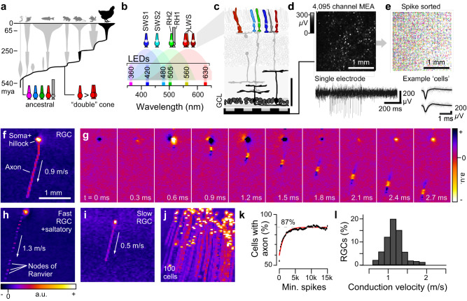
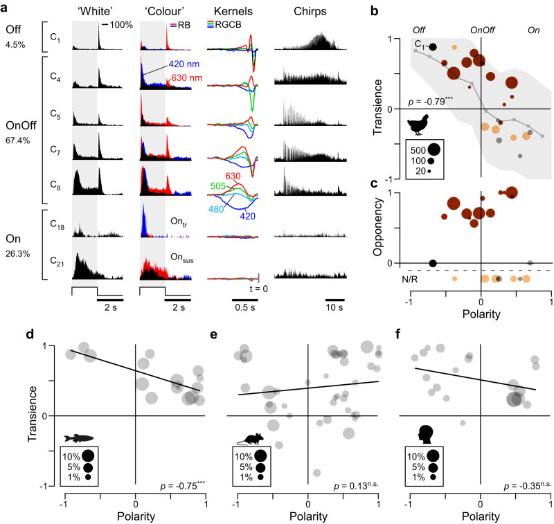
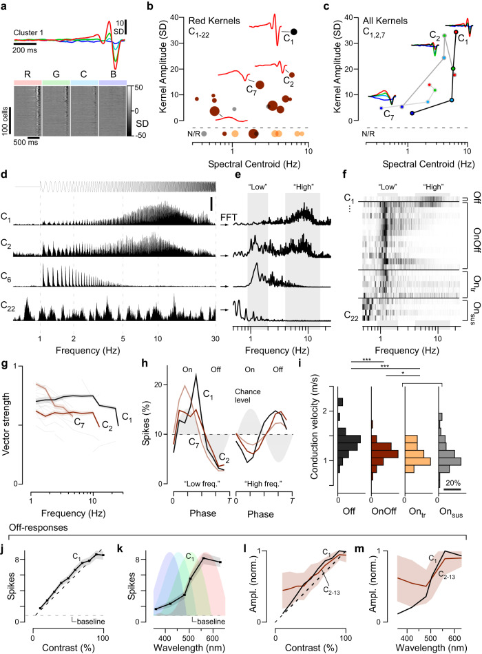
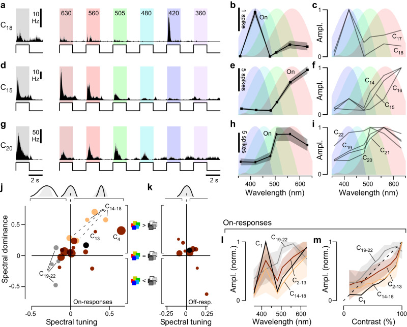
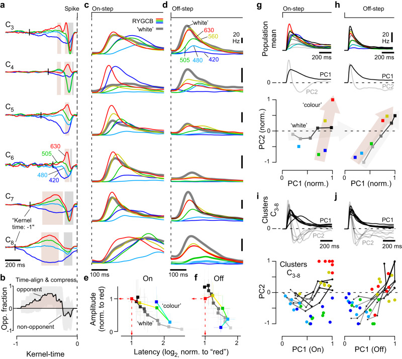
In vertebrate vision, early retinal circuits divide incoming visual information into functionally opposite elementary signals: On and Off, transient and sustained, chromatic and achromatic. Together these signals can yield an efficient representation of the scene for transmission to the brain via the optic nerve. However, this long-standing interpretation of retinal function is based on mammals, and it is unclear whether this functional arrangement is common to all vertebrates. Here we show that male poultry chicks use a fundamentally different strategy to communicate information from the eye to the brain. Rather than using functionally opposite pairs of retinal output channels, chicks encode the polarity, timing, and spectral composition of visual stimuli in a highly correlated manner: fast achromatic information is encoded by Off-circuits, and slow chromatic information overwhelmingly by On-circuits. Moreover, most retinal output channels combine On- and Off-circuits to simultaneously encode, or multiplex, both achromatic and chromatic information. Our results from birds conform to evidence from fish, amphibians, and reptiles which retain the full ancestral complement of four spectral types of cone photoreceptors.


Conflict of interest statement

The authors declare no competing interests.

Figures

Fig. 1
Fig. 1. Recording light-driven spiking activity from the chick retina.
a Phylogenetic tree of extant vertebrates based on ref. , indicating key evolutionary transitions in photoreceptor complements leading to birds. b Summary of birds’ seven types of ciliary photoreceptors and their expressed opsins (top), the respective spectral sensitivity functions of their four cone opsins (shadings), and spectral positions of the six LEDs used for visual stimulation. c Schematic of chicken retina modified from ref. illustrating the multielectrode array (MEA) recoding strategy. GCL, ganglion cell layer. The coloured cells in the top are the photoreceptors, while the dark grey-shaded neurons in the bottom depict retinal ganglion cells (RGCs, the retina’s output neurons), potentially alongside local interneurons called displaced amacrine cells (dACs). d Representative recording frame from the 64 × 64 MEA array, indicating localised activity on a subset of electrodes (top) and example trace from a single electrode (bottom). e Overview of all spike-sorted units detected in an example recording (top) and spike waveforms of two example ‘cells’ (bottom). f Minimum intensity projection across 50 time bins (corresponding to ~3 ms) of a representative electrical image (EI) computed from a single spike sorted unit, revealing the position of the soma, hillock and axon, as indicated. g Time-series from the EI shown in (g), illustrating how the spike travels down the axon towards the optic disc. hj As (f) but for two different spike sorted units (h, i) and for 100 such units superimposed (j). Note that the axonal footprint in (h) is fractionated, indicating saltatory conduction, while the footprints in (f) and (i) are continuous, indicating non-saltatory conduction (cf. ref. ). k Fraction of EIs with a clearly detectable axon (y-axis, Methods) plotted for different subsets of the full EI dataset, staggered by the minimum number of spikes available to compute each EI (x-axis). The asymptote of an exponential fit to this data (red) indicates the presumed fraction of EIs that have an axon independent of the signal quality was ~87%. l Distribution of axonal conduction velocities estimated from all presumed RGCs (n = 842). Source data are provided as a Source Data file.
Fig. 2
Fig. 2. Example light responses.
ad Spiking light responses of four example cells to the battery of presented stimuli, including the 100% contrast ‘white’ (a) and ‘coloured’ steps (b) with centre wavelengths in nm indicated in the top, the chirp stimulus (c) and, correspondingly with (b), the groups of spectral kernels recovered from spectral noise stimulation (d). Solid histograms indicate the trial-averaged means per cell, with spike-rasters beneath showing the individual repeats. Note that in (b) the 6th colour step response (near-UV) is not shown as cells tended to not respond at this wavelength. The full responses are included in the online plotter (see below). Source data are provided as a Source Data file.
Fig. 3
Fig. 3. A tight link between polarity, kinetics, and colour opponency.
a Overview of selected cluster means to the full set of presented stimuli, illustrating some of their systematic differences. For simplicity, only the 100% contrast response is shown for WS, while only the red- (630 nm) and blue-responses (420 nm) are shown for CS. The full set of cluster means are shown in Supplemental Fig. S3. The entire dataset alongside a basic, cluster wise analysis, is interactively plotted and available for download at http://chicken-data.retinal-functomics.net/. b, c Relationships of transience (b) and colour opponency (c) with polarity for all clusters based on their mean 100% contrast WS responses (Methods). Symbol size denotes the number of cells allocated to a cluster as indicated, while colouration indicates the four response groups: Off (black), OnOff (brown), On (orange/grey). Note that On-responses are further divided by the kinetics of their CS-responses into a transient (orange) and a sustained group (grey)—cf. Supplemental Fig. 4a, b. b Further shows the mean ± SD shadings for the same relationship based on all individual cells (light grey). A positive transience index denotes a transient cell, 0 sustained, and negative a temporally increasing response, as evaluated by comparing the peak response in two time-windows following the step transition: 80–160 ms and 240–2000 ms (Methods). df As (b), transience and polarity indices of RGCs found in the retina of larval zebrafish (d, based on ref. ), mice (e, based on ref. ), and humans (f, based on ref. ). Linear correlation tests, two-sided: Chicken: p < 0.001; Zebrafish: p < 0.001; Mouse: 0.41; Human: 0.13. Note that in (df), the colour code from (b) does not apply. For further detail see also Supplemental Fig. S4d–g. Source data are provided as a Source Data file. Human silhouette in (f) from silhouettegarden.com.
Fig. 4
Fig. 4. Off-responses encode achromatic temporal contrast.
a Spectral kernels of the most Off-dominated cluster C1, showing the cluster mean (top) and a heatmap of all constituent cells’ kernels (bottom), as indicated. b, c comparison of kernel amplitudes and kinetics (spectral centroids, Methods), here shown for ‘red’ kernels of all clusters (b), and for the full complement of R, G, C, B kernels for three exemplary clusters (c). df Mean chirp-responses of four example clusters as indicated (d), their corresponding area normalised magnitude squared Fourier transform (e) and heatmap of all clusters’ Fourier transforms (f). “Low” and “High” frequency windows that were used as the basis of computing a High Frequency Index (Methods, Supplemental Fig. 5a, c, d) and for (i) are shaded into the background. g Degree of phase locking at different frequencies for all clusters, quantified as vector strength (means ± s.e.m.). Three exemplary clusters are highlighted with solid lines, the remainder of clusters is plotted faintly in the background. Non-significant entries (Methods) are not shown. h Area-normalised phase histograms (Methods) of three example clusters across two frequency windows as indicated in (e, f) (for all clusters, see Supplemental Fig. 5b). Background shading indicates the phase of the light. i Histograms of axonal conduction velocities computed from electrical images for the four cluster-groups as indicated (cf. Fig. 1l). Wilcoxon Rank Sum Test, 1 tailed: Off vs OnOff: p < 0.001, Off vs. On(tr+sus): p < 0.001; OnOff vs. On(tr+sus): p = 0.041; (For the purposes of statistical comparison, Ontr and Onsus data were combined in view of the relatively small number of Ontr cells that yielded a reliable electrical image due to their generally very low spike counts). j, k Cluster C1 mean ± SEM number of spikes elicited when probed with the WS (j) and CS (k) stimuli. The background shading in (k) indicate the log-transformed spectral sensitivity functions of the chicks’ four cone-opsins—note match of the C1 tuning to the ‘red’ (LWS) opsin. l, m as (j, k), respectively, for all clusters that showed a strong off-component. Shown are means ± SD across all peak-normalised cluster means (Methods) allocated to the OnOff group C2–13 (brown), and the corresponding normalised entries for the only cluster in the Off group C1 (black). Source data are provided as a Source Data file.
Fig. 5
Fig. 5. On-responses encode wavelength information.
ai Mean ± SEM spike-responses to the 100% WS and all six CS stimuli of On-clusters as indicated, showing spike-histograms (a, d, g), spike counts per On-response during CS stimulation (b, e, h), and normalised mean response amplitudes of all On-clusters that exhibited blue- (c) or red-dominated tunings (f), and for those that are broadly tuned (i). j, k Relationship of ‘spectral dominance’ and ‘spectral tuning’ (Methods) for all clusters’ On- (j) and, where applicable, Off-responses (k). cf. Supplemental Fig. 6a, b for a cell-wise plot of the same data. Symbols above the plots indicate spectral width (from left: broader-, equal-, narrower-than-opsin), while symbols to the side indicate a dominant response to ‘coloured’ (top) or ‘white’ (bottom) stimulation. l, m As Fig. 4m, l, respectively, but here shown for On-responses (means ± SD). Note that unlike for Off-responses (Fig. 4), the spectral tuning of On-responses could generally not be captured by a single opsin (l), and contrast-response functions were generally non-linear (m). Source data are provided as a Source Data file.
Fig. 6
Fig. 6. OnOff circuits multiplex spectral and temporal information.
a Example spectral kernels for six of the twelve OnOff clusters as indicated. For each cluster, shadings indicate the parts of the kernels that were classed as either colour opponent (brown) or non-opponent (grey, Methods). The timepoint of each cluster’s onset is indicated by a short vertical line (kernel time: −1). b Mean ± SD ‘kernel-opponency over normalised time’ for all twelve OnOff clusters C2–13, based on the temporal and opponency measures indicated in (a); see Methods for details. On average, OnOff cluster kernels tended to be colour opponent over long timescales (1, brown), but converged onto a non-opponent (−1, brown) period on short time-scales (i.e. closer in time to the spike event at kernel time 0). The time-normalisation was required in view of the very different overall kinetic regimes across clusters. cf Mean On- (c, e) and Off- (d, f) step responses as indicated for the same OnOff clusters listed in (a), illustrating some of their diversity in kinetics and amplitudes. Note that for On-, but not Off-, red-responses tended to exhibit the largest amplitudes and shortest latencies. The summary plots in (e) and (f) show the mean ± SD response amplitudes and latencies of all CS and WS responses for all twelve OnOff clusters, each normalised to their respective red response. g, h Principal component analysis (PCA) of average On- (g) and Off- (h) WS and CS responses across all twelve OnOff clusters. Top: Traces going into the PCA, which comprised all CS responses except UV, which was generally weak, and 5 of the 10 WS responses (every second contrast value, i.e., 100, 80, 60% etc.). middle: First and second principal component, as indicated, and bottom: Peak-normalised loadings (Methods) of each step response onto the two components. Note that for On-, but not Off-, WS and CS step responses followed approximately orthogonal trajectories in this PC space (indicated by the shaded arrows). i, j (as g, h), but computed separately for the six OnOff clusters shown across (a, c, d). By and large, individual OnOff clusters behaved similarly to the population means (g, h). Source data are provided as a Source Data file.
Fig. 7
Fig. 7. Retinal organisation in the context of vertebrate phylogeny.
a Approximate vertebrate phylogeny, indicating key events in the evolution of retinal circuits (based on refs. , ): The split of the visual signal into On- and Off- circuits likely predates the divergence of jawed from jawless species in the early Cambrian, and probably around the same time, an ancestral RH-opsin expressing photoreceptor gave rise to vertebrate rods and green-cones (but see ref. ). Oil droplets are absent in mammals and elasmobranchs, but present in species of fish, amphibians, reptiles and birds, and non-placental mammals—accordingly the mostly likely origin of oil droplets was between the split of cartilaginous and teleost fish, later followed by their loss in early placental mammals. Amphibians further evolved ‘blue’ rods, while early tetrapods evolved the double cone that is still present in extant birds. By contrast, eutherian mammals lost ancestral SWS2 and RH2 single cones, double cones, and oil droplets, while cartilaginous fish lost SWS1 and SWS2 cones (and sharks also lost LWS cones), and their ancestors never had double cones or oil droplets. The resultant maximal cone-complement is indicated for each lineage: RH1 rods (grey), LWS/double cones (red), RH2 cones (green), SWS2 cones (blue), SWS1 cones (pink) and SWS2 rods (faded blue). b Approximate typical anatomical and functional arrangement of retinal circuits in each lineage. The question marks indicate entries that have not been studied. References for each entry are provided in the relevant sections throughout the main text. Frog silhouette in (a) from silhouettegarden.com.

Similar articles

Cited by

References

    1. Wässle H. Parallel processing in the mammalian retina. Nat. Rev. Neurosci. 2004;5:747–757. doi: 10.1038/nrn1497. - DOI - PubMed
    1. Baden T, Euler T, Berens P. Understanding the retinal basis of vision across species. Nat. Rev. Neurosci. 2020;21:5–20. doi: 10.1038/s41583-019-0242-1. - DOI - PubMed
    1. Masland RH. The fundamental plan of the retina. Nat. Neurosci. 2001;4:877–886. doi: 10.1038/nn0901-877. - DOI - PubMed
    1. Westheimer G. The ON-OFF dichotomy in visual processing: from receptors to perception. Prog. Retin. Eye Res. 2007;26:636–648. doi: 10.1016/j.preteyeres.2007.07.003. - DOI - PubMed
    1. Euler T, Haverkamp S, Schubert T, Baden T. Retinal bipolar cells: elementary building blocks of vision. Nat. Rev. Neurosci. 2014;15:507–519. doi: 10.1038/nrn3783. - DOI - PubMed

Publication types