. 2023 Sep 5:12:RP86635.
doi: 10.7554/eLife.86635.

Evidence for adolescent length growth spurts in bonobos and other primates highlights the importance of scaling laws

Affiliations

Evidence for adolescent length growth spurts in bonobos and other primates highlights the importance of scaling laws

Andreas Berghaenel et al. Elife. .

Abstract

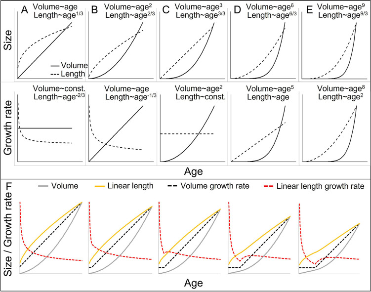
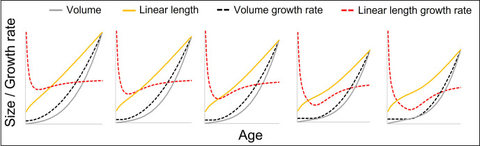
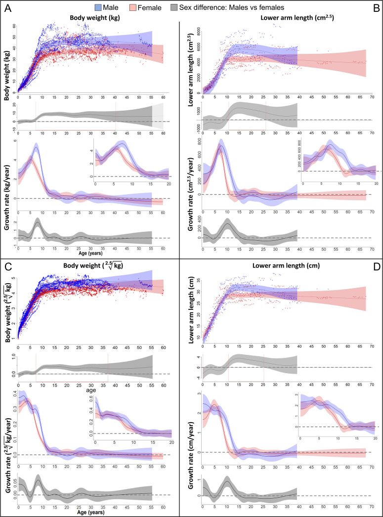
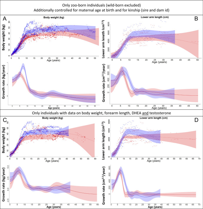
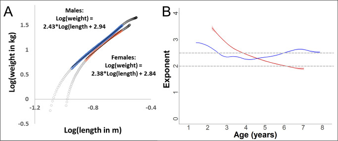
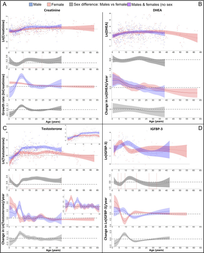
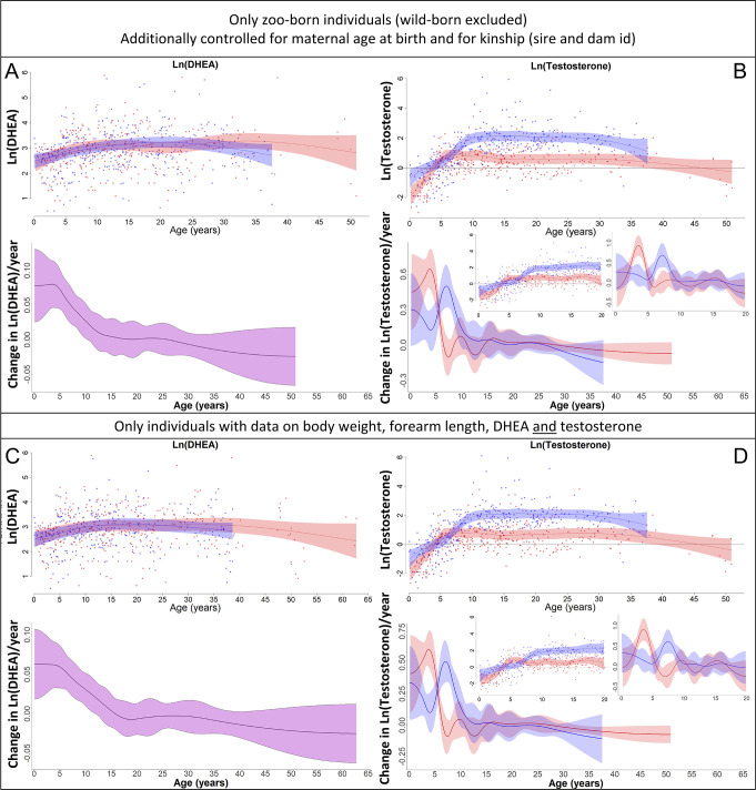
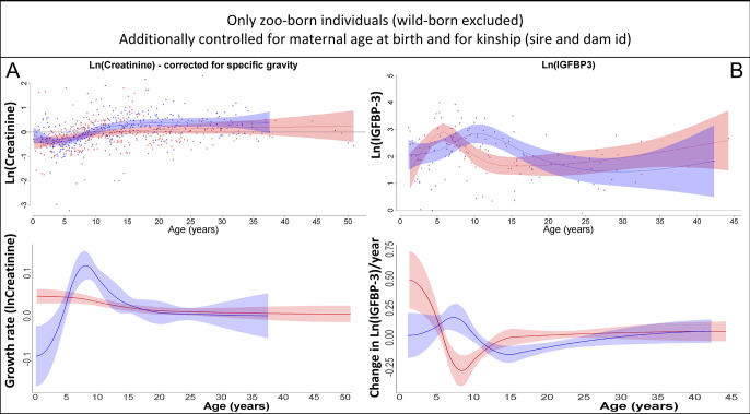
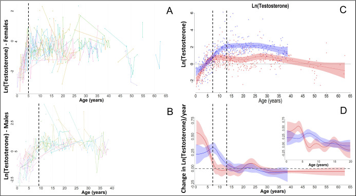
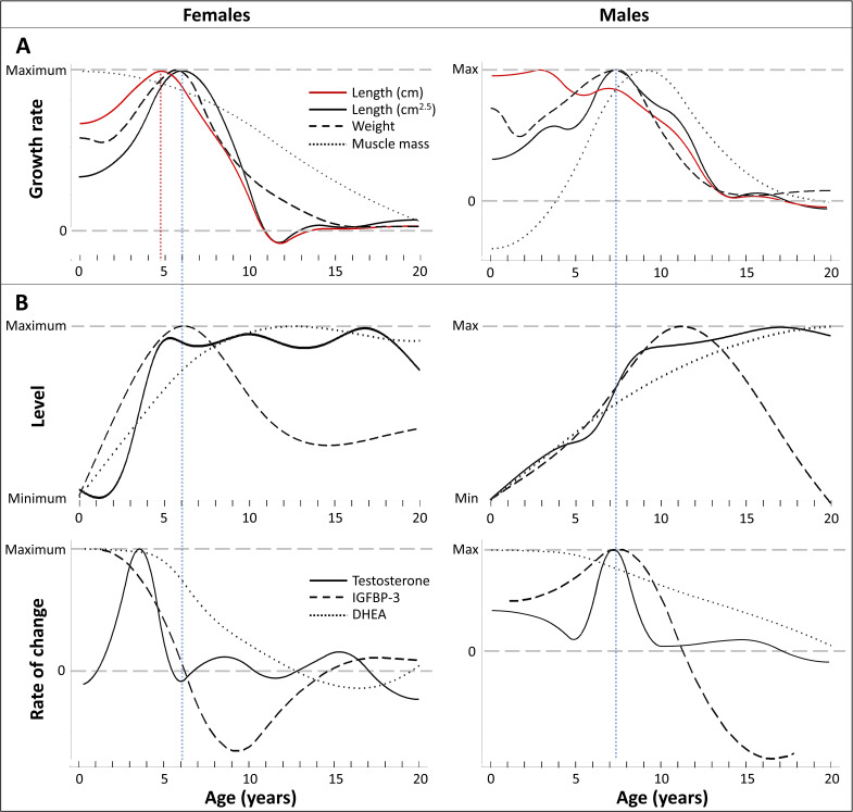
Adolescent growth spurts (GSs) in body length seem to be absent in non-human primates and are considered a distinct human trait. However, this distinction between present and absent length-GSs may reflect a mathematical artefact that makes it arbitrary. We first outline how scaling issues and inappropriate comparisons between length (linear) and weight (volume) growth rates result in misleading interpretations like the absence of length-GSs in non-human primates despite pronounced weight-GSs, or temporal delays between length- and weight-GSs. We then apply a scale-corrected approach to a comprehensive dataset on 258 zoo-housed bonobos that includes weight and length growth as well as several physiological markers related to growth and adolescence. We found pronounced GSs in body weight and length in both sexes. Weight and length growth trajectories corresponded with each other and with patterns of testosterone and insulin-like growth factor-binding protein 3 levels, resembling adolescent GSs in humans. We further re-interpreted published data of non-human primates, which showed that aligned GSs in weight and length exist not only in bonobos. Altogether, our results emphasize the importance of considering scaling laws when interpreting growth curves in general, and further show that pronounced, human-like adolescent length-GSs exist in bonobos and probably also many other non-human primates.

Keywords: Pan paniscus; evolutionary biology; length growth; ontogeny; physiological non-invasive marker; scaling issues; weight growth.


Conflict of interest statement

AB, JS, GH, TD, VB No competing interests declared

Figures

Figure 1.
Figure 1.. Cubic isometric relationship between volume (~weight) and length growth, and likelihood to detect an existing growth spurt (GS) in linear length (schematic).
(A–E) Top/bottom: Absolute size and growth rate (=1st derivation of size). From left to right: Increasingly fast acceleration of volume (~weight) growth and the aligned length growth, from (A) no acceleration (constant volume growth rate and linear increase in volume) through (B) constant acceleration (linear increase in volume growth rate and quadratic increase in volume) to (C) quadratic acceleration of volume growth rate (cubic increase in volume), and (D, E) even faster volume growth acceleration. Due to the cubic relationship, these volume growth rates would align with decreasing (A, B) or constant length growth rates (C), whereas a detectable acceleration in length growth rate may only be found in cases of very fast acceleration in volume growth rate (D, E). Therefore, the current dichotomy between absent and detectable length GSs would only differentiate between (A–C) and (D, E). Another consequence is that, in non-aquatic animals, a cubic relationship is more likely in smaller animals, whereas in larger animals like humans or bonobos, the relationship tends to follow a lower power of 2.5 or even 2 only, as a result from limitation on the bearable weight of a skeletal construction which relates to the sectional area of bones (for more details see e.g., Juul et al., 1995). This means that in case of an equal volume growth acceleration, an aligned acceleration in linear length growth may become more likely detectable in larger animals simply because of the different underlying scaling laws. (F) The above scaling rules lead to further dynamics depending on the temporal overlap of the curves, making length GSs more pronounced and detectable with increasing size (from left to right). A GS in linear length is detectable if the acceleration resulting from the volume-GS exceeds the deceleration in length growth rate that results from the cubic relationship, with the last one becoming weaker with increasing size, respective age. The figure shows how a change from a constant to a linearly accelerating volume growth rate (like in A and B; equal levels of acceleration) results in different levels of acceleration in linear length growth rate depending on the age/size at which this change occurs, from left (change right after birth, only deceleration in length growth rate) (equal to B) to right (change at late age, strong acceleration in length growth rate). Additionally, this figure highlights that even if both volume and linear length show a GS and are perfectly aligned, the linear length growth rate reaches its peak and starts declining again at a time when volume growth rate still increases. See also Figure 1—figure supplement 1 for non-linear acceleration in volume growth rate.
Figure 1—figure supplement 1.
Figure 1—figure supplement 1.. The figure shows how a change from a constant to a quadratically accelerating volume growth rate at a certain body size (identical levels of acceleration) results in different levels of acceleration in linear length growth rate depending on the age (in fact, body size) at which this change occurs, from left (change right after birth at small body size, only slight acceleration in linear length growth rate) to right (change at late age and larger body size, strong acceleration in length growth rate).
Figure 2.
Figure 2.. Growth trajectories in body weight and forearm length, and the importance of comparing them at the relevant dimension.
Fitted values and 95% CIs from Generalized Additive Mixed Models (GAMMs) are shown, implementing variability in trajectories across individuals and zoos. (A, B) Investigating both weight and length growth at the dimension of weight growth reveals pronounced growth spurts (GSs) in both which are strongly aligned with each other in timing and amplitude (see also Figure 4A for easier comparison). (C, D) If instead examined at the scale of one-dimensional length growth, weight, and length growth curves still align with each other but the GSs are not so easily detectable anymore. However, the GS is still evident in female growth, but appears at a younger age than if scale corrected (A, B). The potential fast decrease in growth rate after birth was not covered by linear length data (first half year of age: 2 arm and 854 [729 male] weight measures).
Figure 2—figure supplement 1.
Figure 2—figure supplement 1.. Our results on body weight (left) and forearm length (right) remained the same if (A, B) only zoo-born individuals were considered (which also allowed to additionally control for kinship [dam and sire] and maternal age at birth) or if (C, D) only those individuals were considered for which data on body weight, forearm length, dehydroepiandrosterone (DHEA), and testosterone were available.
Blue = males; red = females. 95% confidence intervals are plotted.
Figure 2—figure supplement 2.
Figure 2—figure supplement 2.. Validation of the scaling relationship between forearm length and body weight during growth in our study.
Since weight and length were not measured pairwise, we used the fitted values from the respective Generalized Additive Mixed Models (GAMMs). The power-exponent of the relationship is calculated as the linear slope of the log–log plot. (A) Log–log plot of weight over length, with data from the growth period (range 0–10 years of age in females and 0–14 years in males, grey circles). During the period of a linear relationship (coloured, blue = males and red = females), the slope (and thus the exponent of the relationship between the non-transformed variables) was 2.4 for both sexes. (B) For the same data used for slope calculation in (A), but with dynamic slope calculation using the first derivative of the GAM-smooth. The exponent for males was relatively stable around 2.5 during this age period, whereas the value decreased in females, reaching about 2.0 towards the end of the growth spurt (see results section, Figures 2—4).
Figure 3.
Figure 3.. Physiological changes during ontogeny: markers of muscle growth (creatinine), adrenarche (dehydroepiandrosterone, DHEA), and adolescence (testosterone and insulin-like growth factor-binding protein 3 [IGFBP-3]).
Fitted values and 95% CIs from Generalized Additive Mixed Models (GAMMs) are shown, which implement variability in trajectories across individuals and zoos. (A) Males showed a pronounced growth spurt (GS) in lean body respective muscle mass, resulting in larger lean body mass in males compared to females where such a GS was not detectable. Be aware though that corrected creatinine values before the age of 3–4 years may be less reliable (Emery Thompson et al., 2012). (B) DHEA levels increased fastest during the first 5 years of life and reached maximal levels at ~15 years. (C) Testosterone levels increased during development in both sexes, but in males, testosterone levels increased longer and reached higher adult levels. They increased fastest at 3.5–4 years in females and 7 years in males. Testosterone levels decreased again after the age of ~30 years of age. (D) IGFBP-3 levels showed a peak of similar height in males and females, occurring at a younger age in females than males.
Figure 3—figure supplement 1.
Figure 3—figure supplement 1.. Our results on dehydroepiandrosterone (DHEA) (left) and testosterone (right) remained the same if (A, B) only zoo-born individuals were considered (which also allowed to additionally control for kinship [dam and sire] and maternal age at birth) or if (C, D) only those individuals were considered for which data on body weight, forearm length, DHEA, and testosterone were available.
Blue = males, red = females. 95% confidence intervals are plotted.
Figure 3—figure supplement 2.
Figure 3—figure supplement 2.. Our results on creatinine (A) and insulin-like growth factor-binding protein 3 (IGFBP-3) (B) remained the same if only zoo-born individuals were considered (which also allowed to additionally control for kinship [dam and sire] and maternal age at birth).
Blue = males, red = females. 95% confidence intervals are plotted.
Figure 3—figure supplement 3.
Figure 3—figure supplement 3.. In our raw data, females and males showed a fast increase in testosterone, as also previously shown for bonobos (Behringer et al., 2014), with females (red) reaching maximal levels around the age of 5, and males (blue) around the age of 9 years.
However, this fast change was not appropriately modelled by our Generalized Additive Mixed Models (GAMMs) if the ‘automatic’ estimation of the smoothing parameters was used, leading to strong oversmoothing and much later ages at which maximal levels were attained, and at which the increase in testosterone levels ceased, in both sexes. Therefore, we applied a fixed smoothing parameter to our testosterone GAMMs of sp = 1, which allowed for higher ‘wiggliness’ and thus faster changes, and which solved the issue.
Figure 4.
Figure 4.. Direct comparison of age trajectories in growth patterns and physiological parameters until the age of 20 years.
All curves are the same as in Figures 2 and 3, and for the respective variability and uncertainty in the trajectories including the occurrence, level, and timing of peaks see the 95% CIs in Figures 2 and 3. Blue and red dotted line: Age at peak growth velocity in cm2.5/year (blue) and in cm/year (red; females only). (A) Change of growth rate over age in weight, forearm length, and lean body respective muscle mass (measured as urinary creatinine). (B) Levels (top) and rate of change (bottom) in urinary testosterone, insulin-like growth factor-binding protein 3 (IGFBP-3) and dehydroepiandrosterone (DHEA) levels.

Update of

  • doi: 10.1101/2023.01.26.525764
  • doi: 10.7554/eLife.86635.1
  • doi: 10.7554/eLife.86635.2

Similar articles

Cited by

References

    1. Abràmoff MD, Magalhães PJ, Ram SJ. Image processing with ImageJ. Biophotonics International. 2004;11:36–42.
    1. Alberti C, Chevenne D, Mercat I, Josserand E, Armoogum-Boizeau P, Tichet J, Léger J. Serum concentrations of insulin-like growth factor (IGF)-1 and IGF binding protein-3 (IGFBP-3), IGF-1/IGFBP-3 ratio, and markers of bone turnover: reference values for French children and adolescents and z-score comparability with other references. Clinical Chemistry. 2011;57:1424–1435. doi: 10.1373/clinchem.2011.169466. - DOI - PubMed
    1. Anestis SF. Testosterone in juvenile and adolescent male chimpanzees (Pan troglodytes): effects of dominance rank, aggression, and behavioral style. American Journal of Physical Anthropology. 2006;130:536–545. doi: 10.1002/ajpa.20387. - DOI - PubMed
    1. Anestis SF, Breakey AA, Beuerlein MM, Bribiescas RG. Specific gravity as an alternative to creatinine for estimating urine concentration in captive and wild chimpanzee (Pan troglodytes) Samples. American Journal of Primatology. 2009;71:130–135. doi: 10.1002/ajp.20631. - DOI - PubMed
    1. Anzà S, Berghänel A, Ostner J, Schülke O. Growth trajectories of wild Assamese macaques (Macaca assamensis) determined from parallel laser photogrammetry. Mammalian Biology. 2022;102:1497–1511. doi: 10.1007/s42991-022-00262-2. - DOI

Publication types