. 2023 Dec 1;44(17):5624-5640.
doi: 10.1002/hbm.26466. Epub 2023 Sep 5.

Multiplexity of human brain oscillations as a personal brain signature

Affiliations

Multiplexity of human brain oscillations as a personal brain signature

Stavros I Dimitriadis et al. Hum Brain Mapp. .

Abstract

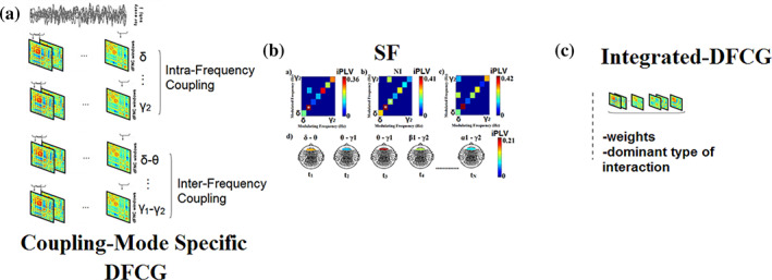
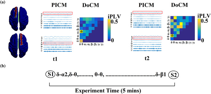
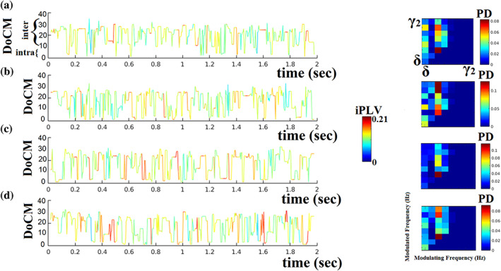
Human individuality is likely underpinned by the constitution of functional brain networks that ensure consistency of each person's cognitive and behavioral profile. These functional networks should, in principle, be detectable by noninvasive neurophysiology. We use a method that enables the detection of dominant frequencies of the interaction between every pair of brain areas at every temporal segment of the recording period, the dominant coupling modes (DoCM). We apply this method to brain oscillations, measured with magnetoencephalography (MEG) at rest in two independent datasets, and show that the spatiotemporal evolution of DoCMs constitutes an individualized brain fingerprint. Based on this successful fingerprinting we suggest that DoCMs are important targets for the investigation of neural correlates of individual psychological parameters and can provide mechanistic insight into the underlying neurophysiological processes, as well as their disturbance in brain diseases.

Keywords: MEG; Multiplexity; chronnectomics; dominant coupling modes; individual fingerprint; resting-state; signal processing; time-varying network analysis.


Conflict of interest statement

The authors declare that they do not have any conflict of interest.

Figures

FIGURE 1
FIGURE 1
Construction of integrated dynamic functional connectivity graphs (iDFCG). (a) We constructed one DFCG per coupling mode for both within‐frequency coupling and cross‐frequency coupling modes (36 in total). Similarly, we constructed 10,000 surrogates DFCG per coupling mode, and assigned a p‐value per each of the 36 coupling modes for every pair of ROIs within a temporal segment. An example of the first three temporal segments from the first subject of the first cohort is illustrated in (b). From this process, we can untangle if two brain regions are functionally connected and if so, which is the preferred dominant coupling mode. (c) The outcome of the surrogate analysis is an iDFCG that preserves both the weight and the dominant type of interaction (SF ‐ Statistical Filtering).
FIGURE 2
FIGURE 2
Determining Dominant Intrinsic Coupling Modes (DoCM). (a) Schematic illustration of the approach employed to identify the DoCM between two AAL atlas ROIs (left superior frontal gyrus, right superior frontal gyrus) for two consecutive 1 s sliding time windows (t 1, t 2) during the resting‐state MEG recording. In this example, the functional interdependence between band‐passed signals from the two virtual sensors was indexed by imaginary Phase Locking (iPLV). In this manner, iPLV was computed between the two virtual sensors either for same‐frequency oscillations (e.g., δ to δ) or between different frequencies (e.g., δ to θ; Potential Intrinsic Coupling Modes [PICM]). Statistical filtering, using surrogate data for reference, was employed to assess whether each iPLV value was significantly different from chance. During t 1 the DoCM reflected significant phase locking between δ and α2 oscillations (indicated by red rectangles) whereas during t 2 the dominant interaction was found between δ and θ oscillations. (b) Burst of DoCM between left superior frontal gyrus and right superior frontal gyrus. This packeting can be thought to group the “letters” contained in the DoCM series to form a neural “word.”, representing a possible integration of many DoCMs (Leinekugel et al, 2002).
FIGURE 3
FIGURE 3
Dynamic reconfiguration of dominant coupling modes for four pairs of ROIs. (a) Right frontal‐superior‐orbital–right parietal‐superior, (b) left frontal‐middle–right parietal‐inferior, (c) left frontal‐middle–right frontal‐middle, and (d) left temporal superior–left frontal superior for subject 1. (a) In the left subplot, color represents the strength of iPLV coupling while the height of the fluctuated time series (y‐axis) codes the dominant intrinsic coupling mode (DoCM) over 36 possible options (8 for intra‐frequency and 28 for cross‐frequency coupling). (b) The 2D matrix is a comodulogram that tabulates the probability distribution (PD) of each dominant coupling mode across the time series presented in (a). For each time series, we plotted the comodulograms which tabulate the probability distribution of dominant coupling modes across intra (main diagonal) and cross‐frequency coupling (off‐diagonal). The total sum of the probability distribution is equal to 1. The horizontal axis refers to the modulating frequencies while the vertical axis refers to the modulated frequencies. From the comodulograms, one can understand that the basic modulators of intrinsic activity are mainly δ, θ, α1, and α2 brain rhythms.
FIGURE 4
FIGURE 4
Step‐wise classification performance (CP) of the brain‐fingerprinting for the 76 selected edges.
FIGURE 5
FIGURE 5
Repeatability of FI across the repeat MEG resting‐state cohort.
FIGURE 6
FIGURE 6
Results of the two‐stage analysis procedure. The upper panel (Stage 1) shows the identification training using 40 participants with repeat resting‐state MEG data. The lower panel (Stage 2) shows the blind matching, or nonmatching, of these 40 people to an independent dataset of 183 people. Panels (a) and (b) show the nodes and connections that were identified as being important DoCM network features for the initial training. In (a), these are plotted on a 3D template brain representation, while in (b), the same connections are shown on a circular representation of the 90 AAL atlas regions. In (c), the distribution of the 76 connections identified as part of the multi‐parametric brain fingerprinting approach to the five sub‐networks is shown. Each color encodes the total number of connections (NC) related to the identified 76 pairs within and between the five sub‐networks. CO, cingulo‐opercular; DMN, default mode network; FP, fronto‐parietal; O, occipital; SM, sensory motor). In (d), the classification performance of each of the same sub‐networks is shown. Each color encodes the classification performance (CP) of the 76 connections integrated within and between the five networks. (e) shows the performance of the matching procedure as a similarity matrix illustrating the summation of log‐likelihood across 76 training discrete Hidden Markov Models (dHMM) models from the first dataset of each subject (x‐axis) and from the second dataset of each subject (y‐axis). (f) shows the performance of the independent matching test as a similarity matrix, showing the sum of log‐likelihoods across 76 training dHMM models from every subject of the test–retest study and each set of 76 tested sequences of every subject from the population study. Yellow pixels in this matrix represent the successful identification of subjects from the first test–retest study that indeed participated in the second study.
FIGURE 7
FIGURE 7
Performance of cross‐experiment identification. For each of the 40 participants in Cohort 1, the sum(LogLikelihood) is plotted for each match to the 183 people in the second cohort. For 18 of the participants, this is a distribution of values between 100 and 1000, representing no match, that is, the algorithm has correctly estimated that these 18 people were not in the second cohort. For 22 of the 40 participants, a single sum(LogLikelihood) is seen that exceeds a value of 1400. This represents a successful match between Cohort 1 and Cohort 2.
FIGURE 8
FIGURE 8
Differentiability scores (da Silva Castanheira et al., 2021), for each of the original 40 participants, when matching is attempted in cohort 2 (N = 183). For those 22 participants present in the second cohort, the mean score is 4.7 ± 0.5. For those 18 participants not present in the second cohort, the score is 1.7 ± 0.1.

Similar articles

Cited by

References

    1. Abrol, A. , Damaraju, E. , Miller, R. L. , Stephen, J. M. , Claus, E. D. , Mayer, A. R. , & Calhoun, V. D. (2017). Replicability of time‐varying connectivity patterns in large resting state fMRI samples. NeuroImage, 163, 160–176. - PMC - PubMed
    1. Amunts, K. , Malikovic, A. , Mohlberg, H. , Schormann, T. , & Zilles, K. (2000). Brodmann's areas 17 and 18 brought into stereotaxic space‐where and how variable? NeuroImage, 11, 66–84. - PubMed
    1. Aru, J. , Aru, J. , Priesemann, V. , Wibral, M. , Lana, L. , Pipa, G. , Singer, W. , & Vicente, R. (2015). Untangling cross‐frequency coupling in neuroscience. Current Opinion in Neurobiology, 31, 51–61. - PubMed
    1. Barch, D. M. , Burgess, G. C. , Harms, M. P. , Petersen, S. E. , Schlaggar, B. L. , Corbetta, M. , Glasser, M. F. , Curtiss, S. , Dixit, S. , Feldt, C. , Nolan, D. , Bryant, E. , Hartley, T. , Footer, O. , Bjork, J. M. , Poldrack, R. , Smith, S. , Johansen‐Berg, H. , Snyder, A. Z. , … WU‐Minn HCP Consortium . (2013). Function in the human connectome: Task‐fMRI and individual differences in behavior. NeuroImage, 80, 169–189. - PMC - PubMed
    1. Başar, E. , Schmiedt‐Fehr, C. , Mathes, B. , Femir, B. , Emek‐Savaş, D. D. , Tülay, E. , Tan, D. , Düzgün, A. , Güntekin, B. , Özerdem, A. , Yener, G. , & Başar‐Eroğlu, C. (2016). What does the broken brain say to the neuroscientist? Oscillations and connectivity in schizophrenia, Alzheimer's disease, and bipolar disorder. International Journal of Psychophysiology, 103, 135–148. - PubMed

Publication types