Controlling brain dynamics: Landscape and transition path for working memory

Abstract

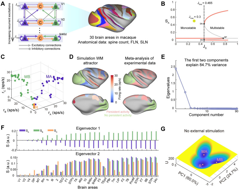
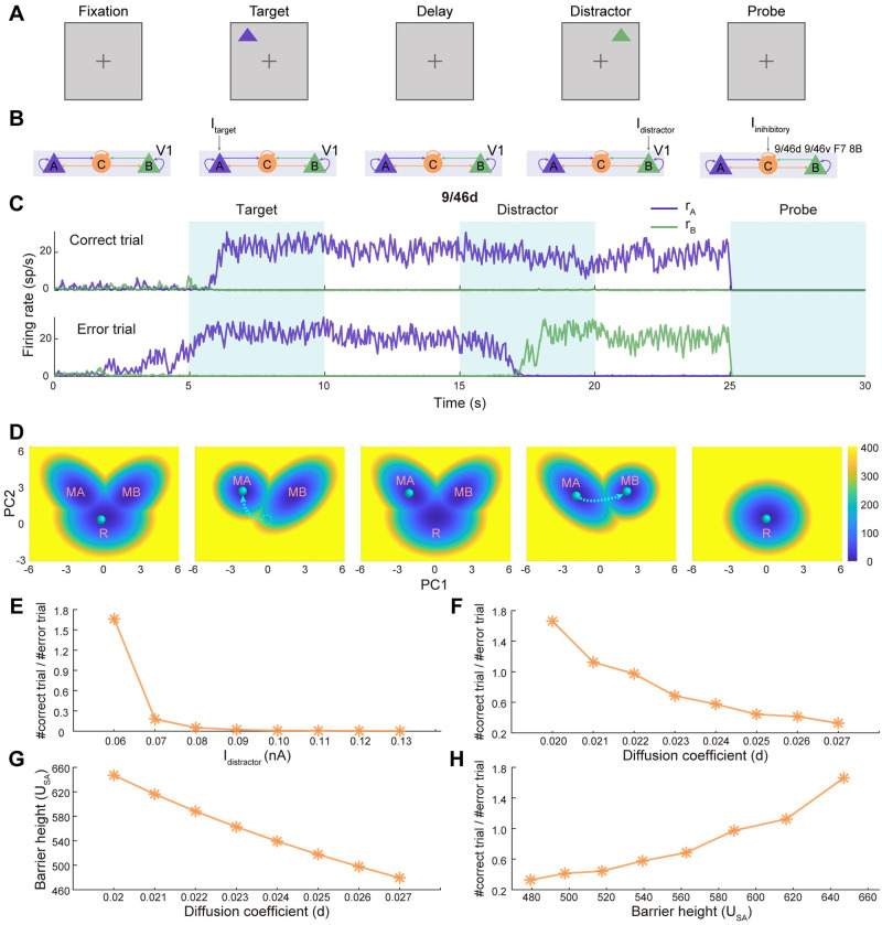
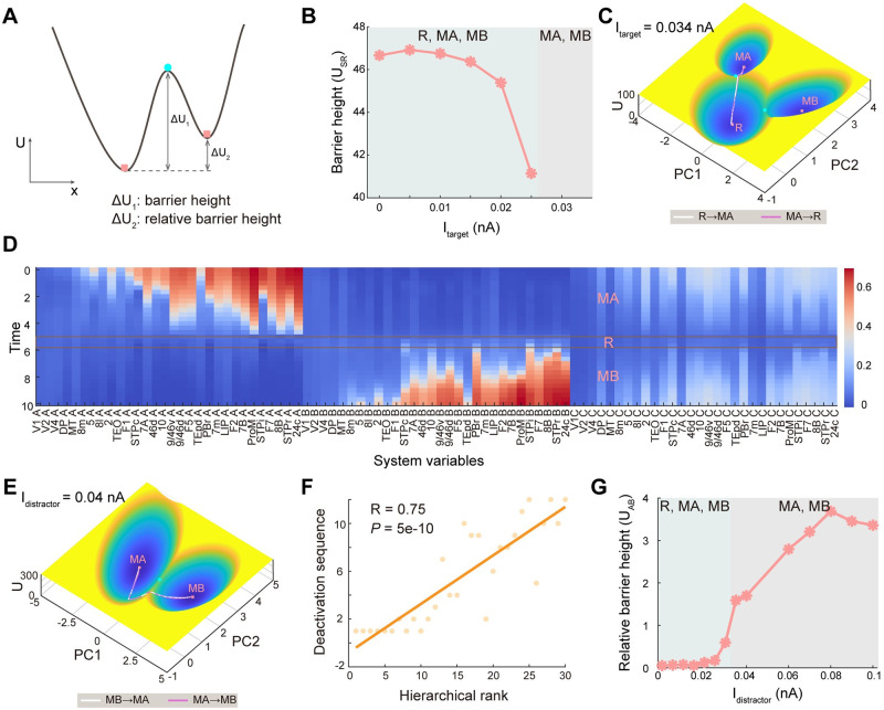
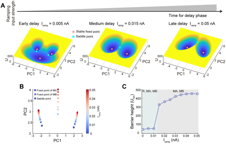
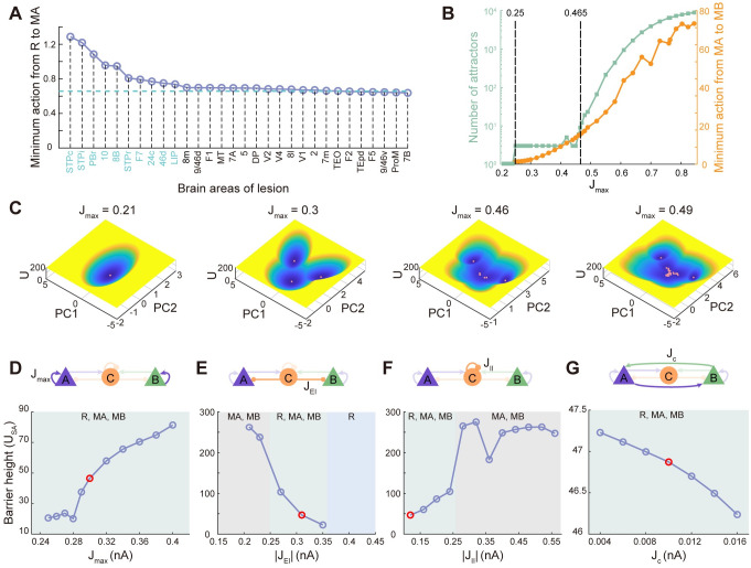
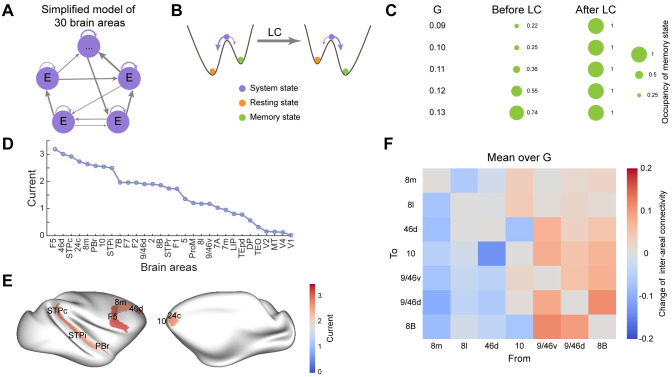
Understanding the underlying dynamical mechanisms of the brain and controlling it is a crucial issue in brain science. The energy landscape and transition path approach provides a possible route to address these challenges. Here, taking working memory as an example, we quantified its landscape based on a large-scale macaque model. The working memory function is governed by the change of landscape and brain-wide state switching in response to the task demands. The kinetic transition path reveals that information flow follows the direction of hierarchical structure. Importantly, we propose a landscape control approach to manipulate brain state transition by modulating external stimulation or inter-areal connectivity, demonstrating the crucial roles of associative areas, especially prefrontal and parietal cortical areas in working memory performance. Our findings provide new insights into the dynamical mechanism of cognitive function, and the landscape control approach helps to develop therapeutic strategies for brain disorders.

Fig 1. The landscape for large-scale working memory system.

(A) The schematic diagram of the computational model of distributed working memory in macaque with 30 brain areas. Each brain area is modeled by two selective excitatory neural populations, labeled as A and B, and one inhibitory population, labeled as C. Each excitatory population has self-excitations and inhibits each other mediated by population C. The inter-areal projections are based on quantitative connectomics data, the fraction of labeled neurons (FLN), and supragranular layered neurons (SLN). For clarity, the cross-couplings between two excitatory populations are not shown. (B) The bifurcation diagram with respect to the recurrent strength (J_S) for the isolated area. In this study, unless specified otherwise, we set the maximum recurrent strength (J_max) as 0.3, lower than the bifurcation point (J_S = 0.465), so that all the brain areas are monostable when isolated. SN: saddle-node, BP: branch point. (C) The three fixed points of the distributed working memory model, resting state (R), memory state encoded by population A (MA), and memory state encoded by population B (MB). (D) There is a strong overlap between the persistent activity of the memory state predicted by the model and the meta-analysis of experimental data [51]. (E) The eigenvalues of the covariance matrix of the probabilistic distribution of system states for dimension reduction of the landscape. The first two components explain 84.7% of the variance. (F) The eigenvectors corresponding to the first two components. (G) The quantified tristable potential landscape after dimension reduction when no external stimulus is applied. Note that the landscape is symmetric along the PC1 axis. The parameters are chosen as default values.

Fig 2. Landscapes explain the working memory function with multistable attractors.

(A-B) The schematic illustration of the visual working memory task. During the fixation phase, no external stimulus is applied. During the target phase, a cue is given, which is modeled as the population A of V1 receiving external current. Then the stimulus is removed and the target is expected to be maintained in working memory against random fluctuations and distractors encoded by population B at the delay epoch. Once the task has been done, the sustained activity should be shut down by delivering excitatory input to the inhibitory populations in four areas (9/46d, 9/46v, F7, 8B), leading to the clearance of working memory. (C) The stochastic neural activity traces of selected areas for correct and error trials (See Fig C in S1 Text for behaviors of all areas). For correct trial, the target stimulus is maintained at delay epoch against distractor. On the contrary, the distractor induces the transition from the stimulus-selective high activity state to the distractor-selective high state for error trial. (D) The corresponding attractor landscapes during different phases of the working memory task. The green ball represents the system state. Before the stimulus onset, the system stays at the resting state (R) with all the populations at low activity. The stimulus changes the landscape topography from tristability to bistability. And the system state transits from R to the dominated target-related memory state (MA). Even after the withdrawal of stimulus and the landscape topography returns back to tristability, the system state keeps staying at MA. However, the presentation of distractor stimulus changes the landscape again and may or may not induce the transition to distractor-related attractor (MB), corresponding error and correct trials, respectively. (E-F) The dependence of the proportion between correct and error trials on the intensity of distractor input and the diffusion coefficient. (G) The barrier height between saddle point and MA (U_SA) versus the diffusion coefficient. (H) The proportion between correct and error trials versus U_SA.

Fig 3. Barrier height and transition path characterize the switching process in working memory.

(A) The illustration for the definition of barrier height (potential difference between the potential at local minimum and saddle point) and relative barrier height (the difference between the two barrier heights) to quantify the stability of attractors. If the system tries to escape from the current attractor, it needs to cross the corresponding barrier. (B) To quantify the difficulty of state transition for the formation of memory, we define the barrier height U_SR as the potential difference between the U_saddle (the potential at the saddle point between R and MA state) and the U_min (the potential at the minimum of R state). The U_SR decreases for higher strength of target stimulus, suggesting the easier formation of memory. (C) The projected transition path with dimension reduction on the landscape between R state and MA state for I_target = 0.034nA. The transition from R to MA represents the formation of memory and the reverse path represents the clearance of memory. (D) The high-dimensional transition path from MA to MB before dimension reduction for a given time T = 10. The X-axis represents the 90 system variables and the Y-axis represents the time points along the transition path. (E) The transition paths between MA and MB for I_distractor = 0.04nA, which pass through the intermediate state R. The transition from MA to MB signifies the change of memory. (F) The deactivation sequence of population A in 30 brain areas shows a high correlation with the anatomical hierarchy as defined by layer-dependent connections [32]. This suggests that the information of distractors flows along the hierarchy, from early sensory areas to association areas. (G) The robustness against distractors during the delay epoch. The increase of relative barrier height between MA and MB as a function of the strength of distractors suggests that MA is becoming more unstable while MB is becoming more stable, thus decreasing the robustness of the system to distractors. R: resting state, MA: memory state encoded by population A, MB: memory state encoded by population B.

Fig 4. Barrier height explains the mechanism of temporal gating of distractors in delay epoch.

(A) The time in the delay epoch is modeled as the non-selective ramping external input to all populations in the system [23, 29, 56]. Three typical landscapes are presented to illustrate the effect of external ramping input on the attraction basins, corresponding to the distractor delivered at the early, medium, and late time of the delay epoch. (B) The two fixed points for memory states moved further away from each other for stronger ramping input I_ramp. (C) The barrier height (U_SA), defined as the potential difference between the saddle point and the fixed point of MA, increases with increasing ramping input. For weaker ramping input, the distractors can more easily push the system state beyond the saddle point and switch from the target-related attractor to the distractor-related attractor.

Fig 5. Connectivities in local circuits underlie working memory performance.

(A) Effects of lesions on individual areas on transition action from spontaneous state to the memory state. The blue dashed line represents no brain lesions. The increase in the transition action for any silenced areas suggests that the formation of distributed working memory becomes harder. The top 10 silenced brain areas which have a strong impact on working memory are consistent with the ‘bowtie hub’ proposed by [33] except LIP. (B) Both the number of attractors and transition action from spontaneous state to memory state increase with increasing maximum recurrent strength (J_max). (C) Four typical landscapes for increasing J_max. (D-G) The robustness against random fluctuations as a function of the barrier height of MA (U_SA), quantifying the network structure. The red dots represent default values.

Fig 6. Landscape control identifies the optimal combination of stimulation targets for the improvement of behavioral performance.

(A) Scheme of simplified distributed working memory model which is composed of 30 interconnected excitatory areas with a gradient of local coupling strengths. (B) An illustration of the landscapes of the simplified model before and after landscape control (LC). Before control, the resting state is deep and stable; after control, the memory state becomes dominant and the system is more inclined to stay in the memory state. (C) The change of the occupancy of memory state before and after LC under different global coupling strengths G. (D) The external stimulation currents of each brain area identified by LC for the improvements of working memory. (E) The top 8 optimal stimulation targets for the improvement of working memory function. The corresponding stimulation currents are indicated by colors. (F) By landscape control, the change of inter-areal connectivity in the prefrontal network can be identified to achieve larger occupancy of desired memory state.

References

1. Christophel TB, Klink PC, Spitzer B, Roelfsema PR, Haynes JD. The distributed nature of working memory. Trends in Cognitive Sciences. 2017;21(2):111–124. doi: 10.1016/j.tics.2016.12.007 - DOI - PubMed
1. Roy DS, Park YG, Kim ME, Zhang Y, Ogawa SK, DiNapoli N, et al.. Brain-wide mapping reveals that engrams for a single memory are distributed across multiple brain regions. Nature Communications. 2022;13(1):1–16. doi: 10.1038/s41467-022-29384-4 - DOI - PMC - PubMed
1. Hopfield JJ. Neural networks and physical systems with emergent collective computational abilities. Proceedings of the National Academy of Sciences. 1982;79(8):2554–2558. doi: 10.1073/pnas.79.8.2554 - DOI - PMC - PubMed
1. Hopfield JJ, Tank DW. Computing with neural circuits: A model. Science. 1986;233(4764):625–633. doi: 10.1126/science.3755256 - DOI - PubMed
1. Izús G, Deza R, Wio H. Exact nonequilibrium potential for the FitzHugh-Nagumo model in the excitable and bistable regimes. Physical Review E. 1998;58(1):93. doi: 10.1103/PhysRevE.58.93 - DOI
Publication types