Block-pulse integrodifference equations

Abstract

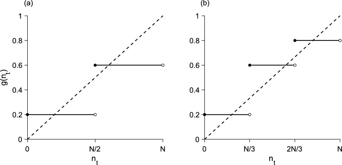
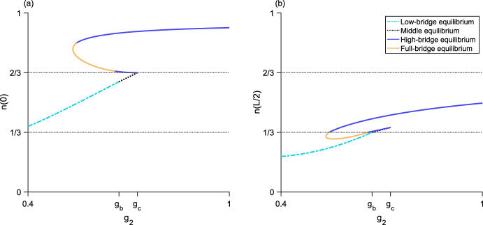
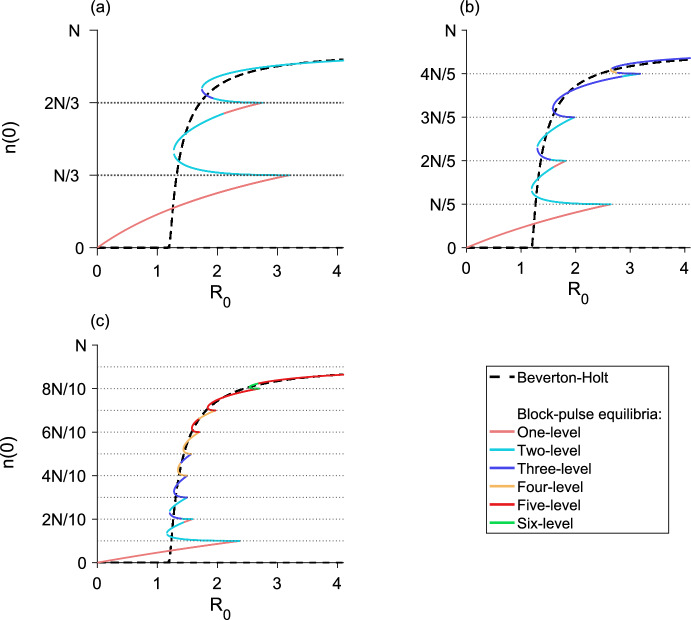
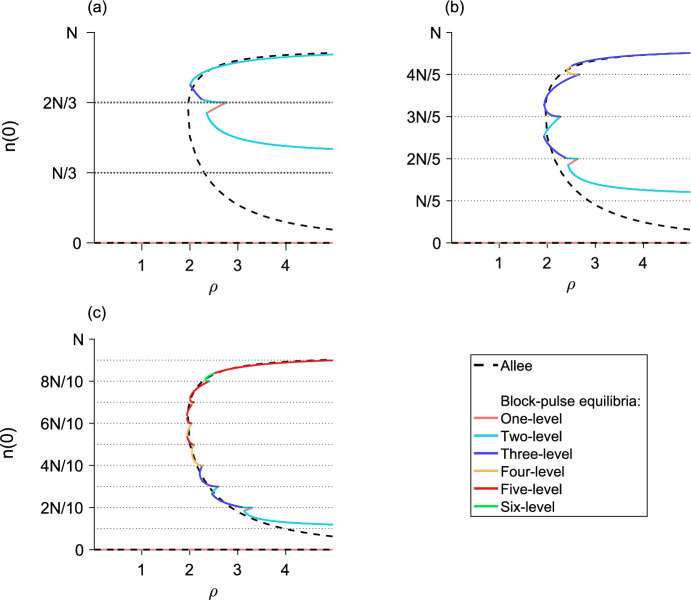
We present a hybrid method for calculating the equilibrium population-distributions of integrodifference equations (IDEs) with strictly increasing growth, for populations that are confined to a finite habitat-patch. This method is based on approximating the growth function of the IDE with a piecewise-constant function, and we call the resulting model a block-pulse IDE. We explicitly write out analytic expressions for the iterates and equilibria of the block-pulse IDEs as sums of cumulative distribution functions. We characterize the dynamics of one-, two-, and three-step block-pulse IDEs, including formal stability analyses, and we explore the bifurcation structure of these models. These simple models display rich dynamics, with numerous fold bifurcations. We then use three-, five-, and ten-step block-pulse IDEs, with a numerical root finder, to approximate models with compensatory Beverton-Holt growth and depensatory, or Allee-effect, growth. Our method provides a good approximation for the equilibrium distributions for compensatory and depensatory growth and offers numerical and analytical advantages over the original growth models.

Keywords: Allee effects; Block-pulse series; Integrodifference equations; Population dynamics; Spatial ecology.

Fig. 1

The Allee growth-function from Eq. (5) with the five-step block-pulse approximation from Eq. (6). Parameters are $\rho =2$, $K=1$, $N=1$, and the five growth-levels are $g_1\approx 0.06$, $g_2\approx 0.33$, $g_3\approx 0.62$, $g_4\approx 0.82$, $g_5\approx 0.95$

Fig. 2

The equilibrium distribution from Eq. (16) (solid) along with the two component cumulative distribution functions (dashed). The left dashed distribution is the first term $F\left(x,+,L,/,2\right)$, the right dashed distribution is the second term $F\left(x,-,L,/,2\right)$. Vertical dotted lines indicate the spatial domain $x\in \left[-,L,/,2,,,L,/,2\right]$. Parameters are $L=1$, $N=1$, $g_1=1$, $\alpha =5$

Fig. 3

Block-pulse growth-functions with a two steps and b three steps. The growth functions (solid) are overlaid on the line of equality (dashed). Parameter values are $N=1$, $g_1=0.2$, $g_2=0.6$, $g_3=0.8$

Fig. 4

Regions of validity in parameter space for the three equilibrium forms. All equilibria are invalid for $g_1\ge g_2$. The low equilibrium is valid inside the dashed region, the high equilibrium is valid inside the dashed-dotted region, and the bridge equilibrium is valid inside the solid region. Vertical dotted lines indicate the boundaries in $g_1$ that lead to different behaviors of the bridge equilibrium. For $g_s<g_1<g_a$, as $g_2$ increases through the lower boundary for the bridge-equilibrium region, a fold bifurcation occurs, resulting in two bridge equilibria for $g_2$ values above the boundary and below $g_b$. At $g_b$, the upper bridge-equilibrium becomes a high equilibrium. Parameter values are $L=0.5$, $N=1$, $\alpha =5$, $g_s\approx 0.17$, $g_a\approx 0.7$, $g_b\approx 1.1$, $g_c\approx 1.4$

Fig. 5

Spatial-threshold mapping from Eq. (30) (solid curve for $r_{1,t}<L/2$) for two different parameter sets with a one fixed point and b two fixed points. The solid horizontal line for $r_{1,t}>L/2$ is an equivalent $r_{1,t}-r_{1,t+1}$ mapping for the high map; as the high map does not depend on $r_{1,t}$ the corresponding $r_{1,t+1}$ is constant regardless of $r_{1,t}$. Using asymptotic Lyapunov stability of the spatial-threshold fixed-points as a proxy for Lyapunov stability of the full equilibrium distributions, in a, the high equilibrium is stable and the bridge equilibrium is unstable; in b the lower bridge-equilibrium is unstable and the upper bridge-equilibrium is stable. Given a particular $r_{1,t}$ in the implicit map from Eq. (30), $r_{1,t+1}$ was computed with the bisection method. Parameter values are $L=0.5$, $N=1$, $\alpha =5$, a $g_1=0.4$, $g_2=1.2$; b $g_1=0.6$, $g_2=1$

Fig. 6

Bifurcation diagram as $g_2$ varies for three different values of $g_1$. The left column (a, c, e) plots the maximum population-density $n\left(0\right)$ and the right column (b, d, f) plots the minimum population-density $n\left(L,/,2\right)$. The horizontal dotted line is the density-threshold value N/2. (a, b), $g_1=0.5$ and $g_1<g_s$; there is a single unstable bridge-equilibrium valid for $g_b<g_2<g_c$. (c, d), $g_1=0.9$ and $g_s<g_1<g_a$; the upper branch of bridge equilibria are stable and the lower branch of bridge equilibria are unstable. (e, f), $g_1=1.2$ and $g_a<g_1<g_2$; there is a single stable bridge-equilibrium valid for $g_1<g_2<g_b$. Both the low and high equilibria are stable. Parameter values are $L=0.25$, $N=1$, $\alpha =5$, $g_s\approx 0.6$, $g_a\approx 1.1$, $g_b\approx 1.4$, $g_c\approx 2.2$

Fig. 7

Regions of validity in a $g_1-g_2$ space and b $g_2-g_3$ space for five of the six equilibrium types of the three-step model. All equilibria are invalid for $g_1\ge g_2$ and $g_2\ge g_3$. a, region of validity is inside: the dashed region for the low equilibrium, the dotted region for the middle equilibrium, and the dashed-dotted region for the low-bridge equilibrium. The high-bridge equilibrium is valid to the left of the vertical solid line. For $g_{s_1}<g_1<g_a$, as $g_2$ increases through the lower border of the region for the low-bridge equilibrium, a fold bifurcation occurs leading to two new low-bridge equilibria. b, region of validity is inside: the dotted region for the middle equilibrium, the dashed region for the high equilibrium, and the solid region for the high-bridge equilibrium. The low-bridge equilibrium is valid above the horizontal dashed-dotted line. For $g_c<g_3<g_d$, as $g_2$ increases through the left boundary of the region for the high-bridge equilibrium, a fold bifurcation occurs leading to two new high-bridge equilibria. Parameter values are $L=0.3$, $N=1$, $\alpha =5$, $g_{s_1}\approx 0.3$, $g_{s_2}\approx 0.6$, $g_a\approx 0.6$, $g_b\approx 0.9$, $g_c\approx 1.3$, $g_d\approx 1.7$, $g_e\approx 1.9$

Fig. 8

Bifurcation diagram as $g_2$ varies for the three-step model. a, the maximum population-density $n\left(0\right)$ of the equilibrium distributions. b, the minimum population-density $n\left(L,/,2\right)$ of the equilibria. Neither the full-bridge nor high equilibria exist for this parameter set, while both the low-bridge and high-bridge equilibria have a fold bifurcation leading to two branches of equilibria. The low and middle equilibria, as well as the upper branches of both low-bridge and high-bridge equilibria, are stable. The lower branches of the low-bridge and high-bridge equilibria are unstable. Parameter values are $L=0.675$, $N=1$, $\alpha =5$, $g_1=0.2$, $g_3=1.2$, $g_{s_1}\approx 0.046$, $g_a\approx 0.41$, $g_b\approx 0.69$, $g_c\approx 0.82$, $g_d\approx 1.38$

Fig. 9

Bifurcation diagram as $g_2$ varies for the three-step model. a, the maximum population-density $n\left(0\right)$ of the equilibrium distributions. b, the minimum population-density $n\left(L,/,2\right)$ of the equilibria. The high equilibrium does not exist for this parameter set, while both the low-bridge and high-bridge equilibria have a fold bifurcation leading to two branches of equilibria. Now, the full-bridge equilibrium is also valid. It exists as a single piece between two segments of the lower branch of the high-bridge equilibrium, where $n\left(L,/,2\right)<N/3$. The low and middle equilibria, as well as the upper branches of both low-bridge and high-bridge equilibria, are stable. The full-bridge equilibrium and lower branches of the low-bridge and high-bridge equilibria are unstable. Parameters are $L=0.8$, $N=1$, $\alpha =5$, $g_1=0.2$, $g_3=1.15$, $g_{s_1}\approx 0.024$, $g_a\approx 0.39$, $g_b\approx 0.68$, $g_c\approx 0.77$, $g_d\approx 1.36$

Fig. 10

Bifurcation diagram as $g_2$ varies for the three-step model. a, the maximum population-density $n\left(0\right)$ of the equilibrium distributions. b, the minimum population-density $n\left(L,/,2\right)$ of the equilibria. Neither the low or high equilibria exist for this parameter set. There is now only one low-bridge equilibrium. A fold bifurcation occurs in the full-bridge equilibrium, and there are two branches of high-bridge equilibria. The middle equilibrium and low-bridge equilibrium, as well as the upper branches of both high-bridge and full-bridge equilibria, are stable. The lower branches of the high-bridge and full-bridge equilibria are unstable. Parameters are $L=1$, $N=1$, $\alpha =5$, $g_1=0.4$, $g_3=1$, $g_a\approx 0.36$, $g_b\approx 0.67$, $g_c\approx 0.73$, $g_d\approx 1.34$

Fig. 11

Bifurcation diagram as $g_2$ varies for the three-step model. a, the maximum population-density $n\left(0\right)$ of the equilibrium distributions. b, the minimum population-density $n\left(L,/,2\right)$ of the equilibria. The high equilibrium does not exist for this parameter set. There is only one each of the low-bridge, high-bridge, and full-bridge equilibria. The low and middle equilibria are stable. The low-bridge, high-bridge, and full-bridge equilibria are unstable. Parameter values are $L=1$, $N=1$, $\alpha =5$, $g_1=0.005$, $g_3=1.5$, $g_{s_1}\approx 0.009$, $g_a\approx 0.36$, $g_b\approx 0.67$, $g_c\approx 0.73$, $g_d\approx 1.34$

Fig. 12

Regions of validity in a $g_1-g_2$ space and b $g_2-g_3$ space for the three-step model, with the region where the high-bridge and full-bridge equilibria meet. All equilibria are invalid for $g_1\ge g_2$ and $g_2\ge g_3$. A fold bifurcation occurs in the high-bridge equilibrium; for larger L the fold bifurcation may occur in the full-bridge equilibrium. a, the full-bridge equilibrium may be valid for $g_2$ below the nearly horizontal solid line. b, the high-bridge equilibrium is valid inside the outer solid region. The inner solid curve marks the boundary where the full-bridge equilibrium meets the high-bridge equilibrium. The full-bridge equilibrium exists inside the inner solid region. For fixed $g_3$, increasing $g_2$ through the left boundary of the region for the full-bridge equilibrium corresponds to the high-bridge transitioning to a full-bridge equilibrium. As $g_2$ increases through the right boundary of the region for the full-bridge equilibrium, there is a transition back into a high-bridge equilibrium. For this domain length, the high equilibrium is not valid. Parameter values are $L=0.675$, $N=1$, $\alpha =5$, $g_{s_1}\approx 0.05$, $g_{s_2}\approx 0.09$, $g_a\approx 0.4$, $g_b\approx 0.7$, $g_c\approx 0.8$, $g_d\approx 1.4$

Fig. 13

The maximum population-density as $R_0$ varies for the Beverton–Holt model (dashed) compared to a a three-step block-pulse model, b five-step block-pulse model, and c ten-step block-pulse model. All block-pulse models are shown with solid lines; p-level equilibria are distinguished from each other for each $p=1,2,\dots ,m$. The Beverton–Holt model has a stable trivial equilibrium until just past $R_0=1$; a transcritical bifurcation occurs as a positive stable branch of nontrivial equilibria emerges and the trivial branch of equilibria becomes unstable. In the block-pulse models, the lower branch of each fold bifurcation is unstable while the upper branches are stable, so that stability alternates. Horizontal dotted lines indicate the density thresholds for each block-pulse model. Parameter values are $L=1$, $N=1$, $\alpha =5$, $K=1$

Fig. 14

The maximum population-density as $\rho$ varies for an Allee-effect growth-model (dashed) compared to a a three-step block-pulse model, b five-step block-pulse model, and c ten-step block-pulse model. All block-pulse models are shown with solid lines; p-level equilibria are distinguished from each other for each $p=1,2,\dots ,m$. The lower branch of nontrivial Allee equilibria is unstable; the trivial and upper nontrivial branch of equilibria are stable. In the block-pulse models, for each fold bifurcation, the resulting lower branch is unstable and upper branch is stable, so that the lowest and highest branches of equilibria are stable, and stability alternates. Horizontal dotted lines indicate the density thresholds for each block-pulse model. Parameter values are $L=1$, $N=1$, $\alpha =5$, $K=1$

Fig. 15

The maximum population-density as $\rho$ varies for an Allee-effect growth-model (dashed) compared to a a three-step block-pulse model, b five-step block-pulse model, and c ten-step block-pulse model. For the block-pulse models, we have set $g_1=0$ to allow for the possibility of extinction. All block-pulse models are shown with solid lines; p-level equilibria are distinguished from each other for each $p=1,2,\dots ,m$. The lower branch of nontrivial Allee equilibria is unstable; the trivial and upper nontrivial branch of equilibria are stable. In the block-pulse models, for each fold bifurcation, the resulting lower branch is unstable and upper branch is stable, so that the lowest and highest branches of equilibria are stable, and stability alternates. Horizontal dotted lines indicate the density thresholds for each block-pulse model. Parameter values are $L=1$, $N=1$, $\alpha =5$, $K=1$

Fig. 16

The maximum population-density as L varies for a ten-step block-pulse model with a a Gaussian, b Laplace, c Cauchy dispersal kernel, where $\rho =2.2$. In d, the critical patch-size for population persistence is shown for the three dispersal kernels for varying growth-parameters $\rho$. To compare the three kernels, we used the same median absolute deviation (MAD) as a measure of dispersion. Parameters values are $N=1$, $K=1$, $\alpha =5$, $\eta =0.05$, $\text{MAD}=0.1386$

Fig. 17

The full spatial equilibrium-distributions of the original Allee model compared to the block-pulse model, using the Laplace kernel, for $\rho =2.2$ and $L=2$. For the block-pulse model, these are the full equilibrium-distributions corresponding to the maximum population-densities at $L=2$ shown in Fig. 16b. Stable equilibria are shown with solid curves; unstable equilibria are shown with dashed curves. Other parameter values are $N=1$, $K=1$, $\alpha =5$

References

1. Allee WC, Park O, Emerson AE, Park T, Schmidt KP. Principles of animal ecology. Philadelphia: Saunders Company; 1949.
1. Andersen M. Properties of some density-dependent integrodifference equation population models. Math Biosci. 1991;104:135–157. - PubMed
1. Apostol TM. Mathematical analysis. 2. Reading: Addison-Wesley Publishing Company; 1974.
1. Babolian E, Masouri Z, Hatamzadeh-Varmazyar S. New direct method to solve nonlinear Volterra–Fredholm integral and integro-differential equations using operational matrix with block-pulse functions. Prog Electromagn Res B. 2008;8:59–76.
1. Balcı MA, Sezer M. Hybrid Euler–Taylor matrix method for solving of generalized linear Fredholm integro-differential difference equations. Appl Math Comput. 2016;273:33–41.
LinkOut - more resources