Causes and consequences of child growth faltering in low-resource settings

Abstract

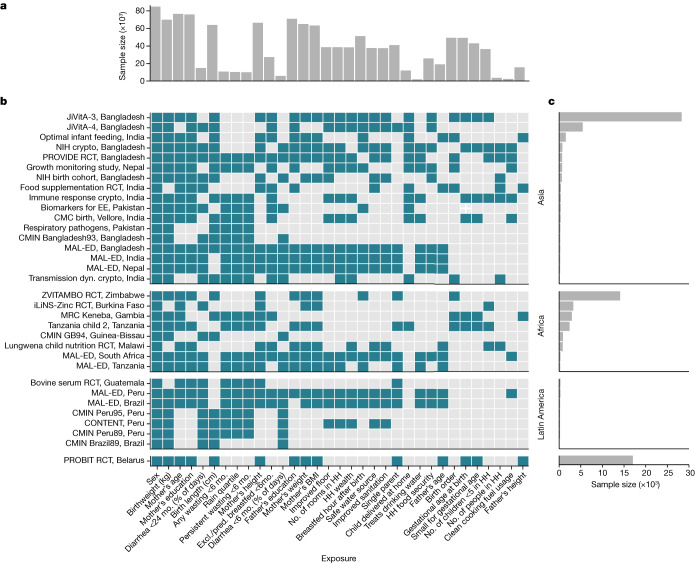
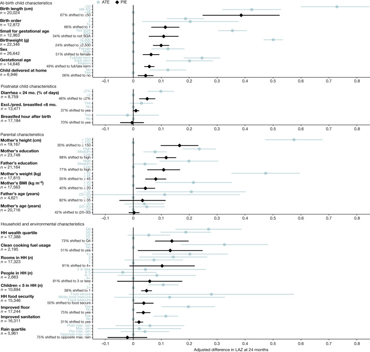
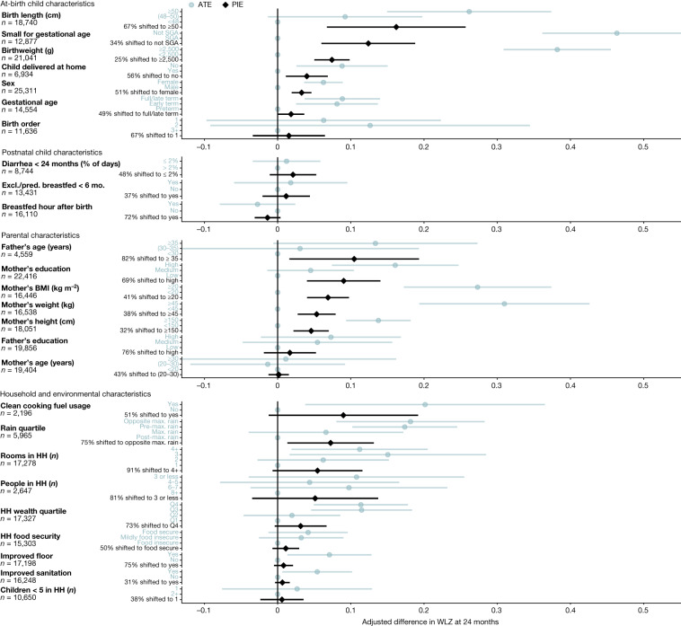
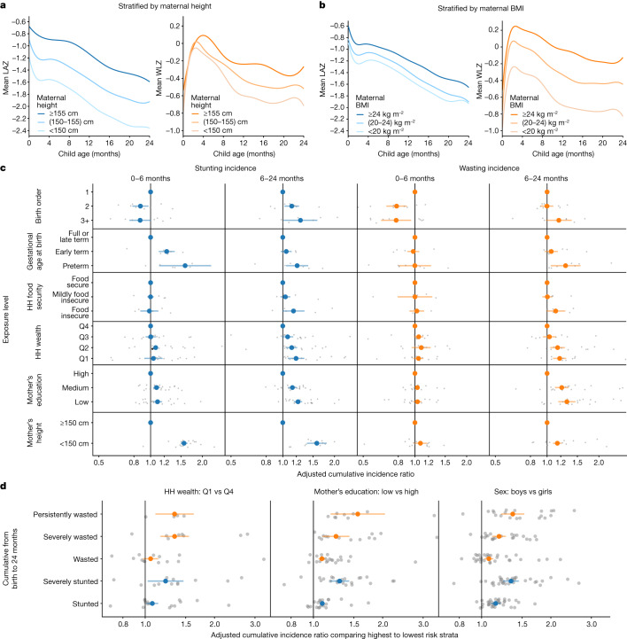
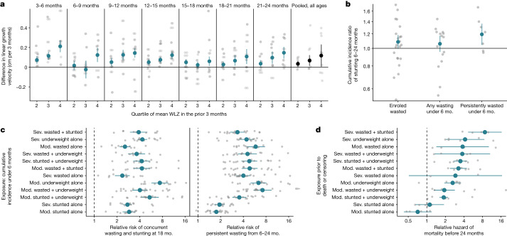
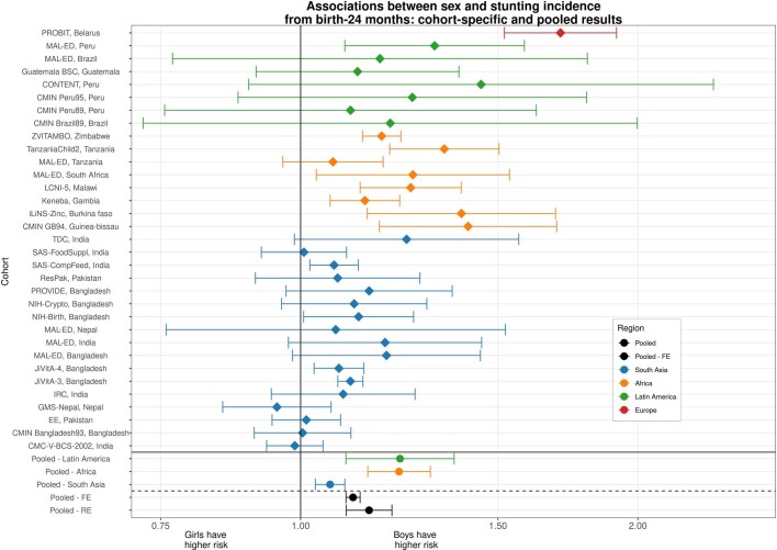
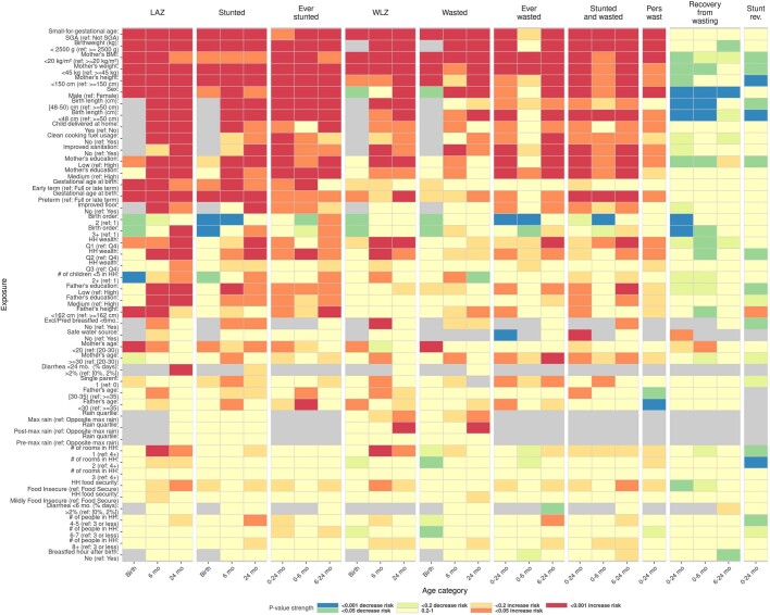
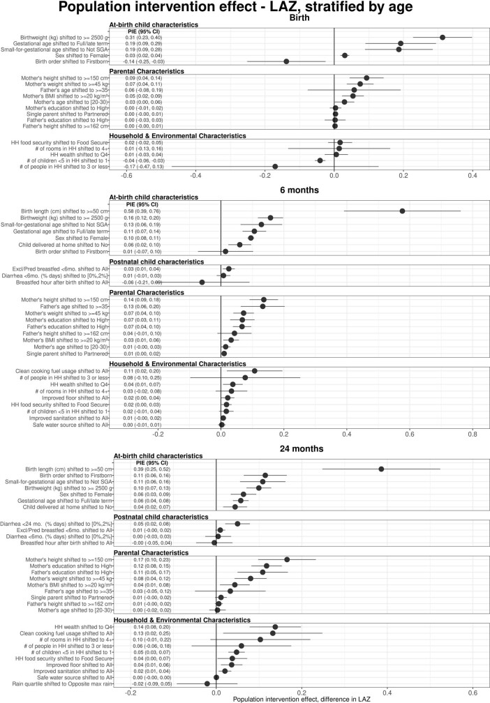
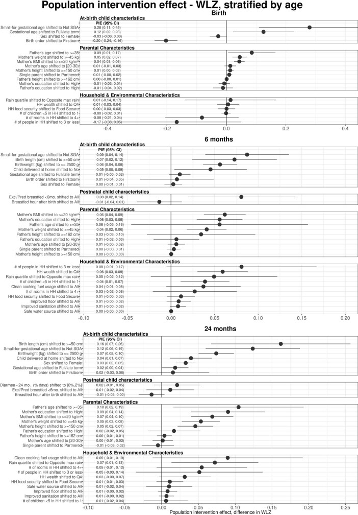
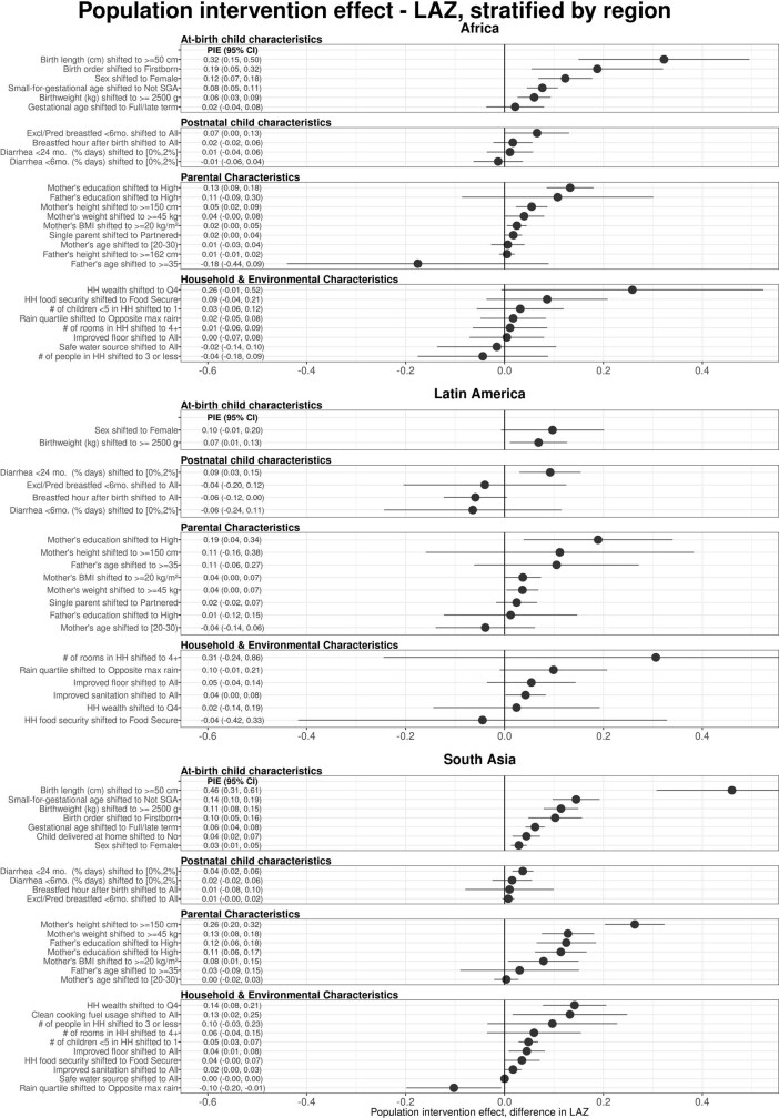
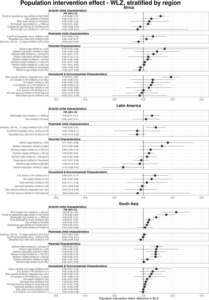
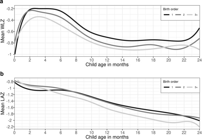
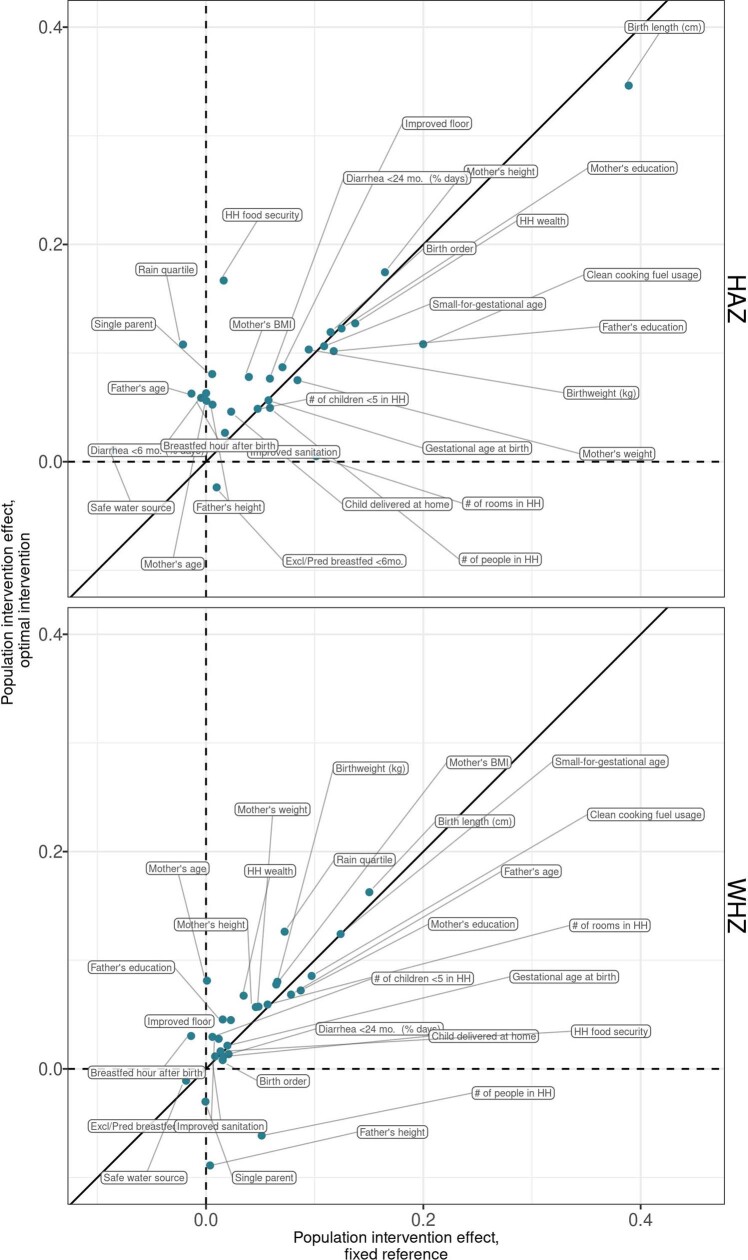
Growth faltering in children (low length for age or low weight for length) during the first 1,000 days of life (from conception to 2 years of age) influences short-term and long-term health and survival^1,2. Interventions such as nutritional supplementation during pregnancy and the postnatal period could help prevent growth faltering, but programmatic action has been insufficient to eliminate the high burden of stunting and wasting in low- and middle-income countries. Identification of age windows and population subgroups on which to focus will benefit future preventive efforts. Here we use a population intervention effects analysis of 33 longitudinal cohorts (83,671 children, 662,763 measurements) and 30 separate exposures to show that improving maternal anthropometry and child condition at birth accounted for population increases in length-for-age z-scores of up to 0.40 and weight-for-length z-scores of up to 0.15 by 24 months of age. Boys had consistently higher risk of all forms of growth faltering than girls. Early postnatal growth faltering predisposed children to subsequent and persistent growth faltering. Children with multiple growth deficits exhibited higher mortality rates from birth to 2 years of age than children without growth deficits (hazard ratios 1.9 to 8.7). The importance of prenatal causes and severe consequences for children who experienced early growth faltering support a focus on pre-conception and pregnancy as a key opportunity for new preventive interventions.

Fig. 1. Cohort sample sizes and measured exposures.

a, The total number of children with each measured exposure, sorted from left to right by the number of cohorts measuring the exposure. b, The presence of 30 exposure variables in the ki data by within each included cohort. Cohorts are sorted by geographic region and sample size. Details of the cohorts are provided in Extended Data Table 1. CMC, Christian Medical College; Crypto, Cryptosporidium; dyn., dynamics; EE, Environmental Enteropathy; Excl., exclusively; HH, household; NIH, National Institute of Health; mo., months; pred., predominantly; RCT, randomized controlled trial. c, The number of child anthropometry observations contributed by each cohort.

Fig. 2. Population intervention effects and mean differences for child, parental, and household exposures on LAZ at 24 months of age.

Adjusted mean differences in average treatment effects (ATEs) (blue) between the labelled higher-risk level of exposures and the reference level (grey dot on the vertical line), and population intervention effects (PIEs) (black), the estimated difference in LAZ after shifting exposure levels for all children to the reference level. The number of children that contributed to each analysis is listed for each exposure. Labels on the y axis indicate the level of exposure used to estimate the ATE (blue) or the percentage of the population shifted to the lowest-risk level to estimate the PIE (black). Cohort-specific estimates were adjusted for all measured confounders using ensemble machine learning and targeted maximum-likelihood estimation (TMLE) and then pooled using random effects (Methods). Estimates are shown only for exposures measured in at least four cohorts. Max. maximum; Q, quartile; SGA, small for gestational age.

Fig. 3. PIEs and mean differences for child, parental and household exposures on WLZ at 24 months of age.

Adjusted mean differences in ATEs (blue) between the labelled higher-risk level of exposures and the reference level (grey dot on vertical line), and PIEs (black), the estimated difference in WLZ after shifting exposure levels for all children to the reference level. The number of children that contributed to each analysis is listed for each exposure. Labels on the y axis indicate the level of exposure used to estimate the ATE (blue) or the percentage of the population shifted to the lowest-risk level to estimate the PIE (black). Cohort-specific estimates were adjusted for all measured confounders using ensemble machine learning and targeted maximum-likelihood estimation (TMLE) and then pooled using random effects (Methods). Estimates are shown only for exposures measured in at least four cohorts.

Fig. 4. Effect of key exposures on the trajectories, timing and severity of child growth faltering.

a, Child LAZ and WLZ trajectories stratified by maternal height (n = 413,921 measurements, 65,061 children, 20 studies). b, Child LAZ and WLZ stratified by maternal BMI (n = 373,382 measurements, 61,933 children, 17 studies). Growth trajectories stratified by all other examined risk factors are available in Supplementary Note 5. c, Associations between key exposures and cumulative wasting incidence, stratified by age of the child during wasting incidence. Grey dots indicate cohort-specific estimates. d, Associations between key exposures and growth faltering of different severities. Cumulative incidence ratios compare the highest and lowest-risk categories of each exposure, as indicated above each graph. Grey dots indicate cohort-specific estimates.

Fig. 5. Growth faltering in early life increases risk of more severe growth faltering and mortality.

a, Adjusted differences in linear growth velocity across three-month age bands by quartile of WLZ in the preceding three months. The reference group (horizontal line) comprises children in the first quartile of WLZ in each age stratum. Far right, pooled estimates unstratified by child age. Velocity was calculated from the closest measurements within 14 days of the start and end of the age period. b, Relative risk of stunting onset between 6 and 24 months of age among children who experienced measures of early wasting before 6 months of age compared with children who did not. Grey dots indicate cohort-specific estimates. c, Association between cumulative incidence of mutually exclusive definitions of growth faltering before 6 months of age and persistent wasting from 6 to 24 months of age (33 cohorts, 6,046 cases and 68,645 children) or concurrent wasting and stunting at 18 months of age (31 cohorts, 1,447 cases, and 22,565 children). The reference group (vertical dashed line) comprises children with no measure of growth failure. Growth faltering definitions are sorted by estimates in d. d, Hazard ratios between mutually exclusive definitions of growth faltering and mortality before 24 months of age (8 cohorts, 1,689 deaths with known age of death, and 63,812 children). The reference group (vertical dashed line) comprises children with no measure of growth failure. Grey dots indicate cohort-specific estimates. Mod, moderately; sev, severely.

Extended Data Fig. 1. Example forest plot of cohort-specific and pooled parameter estimates.

Cohort-specific estimates of the cumulative incidence ratio of stunting are plotted on each row, comparing the risk of any stunting from birth to 24 months among boys compared to a reference level of girls. Below the solid horizontal line are region-specific pooled measures of association, pooled using random-effects models. Below the dashed line are overall pooled measures of association, comparing pooling using random or fixed effects models. The primary results reported throughout the manuscript are overall (not region stratified) estimates pooled using random effects models.

Extended Data Fig. 2. Heatmap of significance and direction across exposure-outcome combinations.

The heatmap shows the significance and direction of estimates through the cell colors, separated across primary outcomes by child age. Red and orange cells are exposures where the outcome is estimated have an increased probability of occurring compared to the reference level (harmful exposures except for recovery outcomes), while blue and green cells are exposures associated with a decreased probability of the outcome (protective exposures except for recovery outcomes). The outcomes are labeled at the top of the columns, with each set of three columns the set of three ages analyzed for that outcome. Each row is a level of an exposure variable, with reference levels excluded. Rows are sorted top to bottom by increasing average p-value. Grey cells denote comparisons that were not estimated or could not be estimated because of data sparsity in the exposure-outcome combination. All point estimates and confidence intervals for exposure-outcome pairs with P-values plotted in this figure are viewable online in Supplimentary Note 7.

Extended Data Fig. 3. Age-stratified population intervention effects in length-for-age Z-scores.

Exposures, rank ordered by population intervention effect on child LAZ, stratified by the age of the child at the time of anthropometry measurement. The population intervention effect is the expected difference in mean Z-score if all children had the reference level of the exposure rather than the observed exposure distribution. Reference levels are printed in the exposure label. Cohort-specific estimates were adjusted for all measured confounders using ensemble machine learning and TMLE, and then pooled using random effects (Methods). Estimates are shown only for exposures measured in at least 4 cohorts.

Extended Data Fig. 4. Age-stratified population intervention effects in weight-for-length Z-scores.

Exposures, rank ordered by population intervention effects on child WLZ, stratified by the age of the child at the time of anthropometry measurement. The population intervention effect is the expected difference in population mean Z-score if all children had the reference level of the exposure rather than the observed distribution. For all plots, reference levels are printed next to the name of the exposure. Cohort-specific estimates were adjusted for all measured confounders using ensemble machine learning and TMLE, and then pooled using random effects (Methods). Estimates are shown only for exposures measured in at least 4 cohorts.

Extended Data Fig. 5. Mediation of parental anthropometry effects by birth size on child Z-scores at 24 months.

Mediating effect of adjusting for birth anthropometry and at-birth characteristics on the estimated Z-score differences between levels of parental anthropometry. Primary estimates were adjusted for all other measured exposures not on the causal pathway, while the mediation analysis estimates were additionally adjusted for birthweight, birth length, gestational age at birth, birth order, small-for-gestational age status, and home vs. hospital delivery. Only estimates from cohorts measuring at least 3 of the 6 at-birth characteristics were used to estimate the pooled Z-score differences (n = 6 cohorts, 17,124 observations). Mediation estimates were slightly attenuated toward the null, and only in the case of maternal height and child WLZ were they statistically different from the primary analysis. These results imply that the causal pathway between parental anthropometry and growth faltering operates through its effect on birth size, but most of the effect is through other pathways.

Extended Data Fig. 6. Rank-ordered associations between child, parental, and household characteristics and adjusted relative risks or population attributable fractions of stunting by age 24 months.

Blue points in the left panel show adjusted cumulative incidence ratios (CIRs) between higher-risk exposure levels and reference levels, and black points in the right panel show population attributable fractions (PAFs), the estimated proportion of the risk in the whole population that would be removed if the exposure were set to its indicated reference level. The number of children that contributed to each analysis is listed by exposure. The colored Y-axis label is either the level of exposure contrasted against the reference level to estimate the CIR, or the percent of the population shifted to the lowest-risk level to estimate the PAF. For at-birth exposures, at-birth stunting and wasting were excluded to focus on incidence of new (postnatal) cases, and for postnatal exposures (breastfeeding practice and diarrheal disease), the cumulative incidence of stunting from 6–24 months was used. Cohort-specific estimates were adjusted for all measured confounders using ensemble machine learning and TMLE, and then pooled using random effects (Methods). Estimates are shown only for exposures measured in at least 4 studies.

Extended Data Fig. 7. Rank-ordered associations between child, parental, and household characteristics and adjusted relative risks or population attributable fractions of wasting by age 24 months.

Blue points in the left panel show adjusted cumulative incidence ratios (CIRs) between higher-risk exposure levels and reference levels, and black points in the right panel show population attributable fractions (PAFs), the estimated proportion of the risk in the whole population that would be removed if the exposure were set to its indicated reference level. The number of children that contributed to each analysis is listed by exposure. The colored Y-axis label is either the level of exposure contrasted against the reference level to estimate the CIR, or the percent of the population shifted to the lowest-risk level to estimate the PAF. For at-birth exposures, at-birth stunting and wasting were excluded, and for postnatal exposures (breastfeeding practice and diarrheal disease), the cumulative incidence of wasting from 6-24 months was used. Cohort-specific estimates were adjusted for all measured confounders using ensemble machine learning and TMLE, and then pooled using random effects (Methods). Estimates are shown only for exposures measured in at least 4 studies. The PAF for diarrhea under 6 months was not calculable or plotted due to the unexpected CIR <1 for estimated higher diarrheal disease burden.

Extended Data Fig. 8. Regionally-stratified population intervention effects for length-for-age Z-scores at age 24 months.

Exposures, rank ordered by population intervention effect on child length-for-age z-score (LAZ) at age 24 months, stratified by region. The population intervention effect is the expected difference in population mean Z-score if all children had the reference level of the exposure rather than the observed distribution. For all plots, reference levels are printed next to the name of the exposure. Cohort-specific estimates were adjusted for all measured confounders using ensemble machine learning and TMLE, and then pooled using random effects (Methods). Estimates are shown only for exposures measured in at least 4 cohorts.

Extended Data Fig. 9. Regionally-stratified population intervention effects for weight-for-length Z-scores at age 24 months.

Exposures, rank ordered by population attributable difference on child weight-for-length z-score (WLZ) at age 24 months, stratified by region. The population intervention effect is the expected difference in population mean Z-score if all children had the reference level of the exposure rather than the observed distribution. For all plots, reference levels are printed next to the name of the exposure. Cohort-specific estimates were adjusted for all measured confounders using ensemble machine learning and TMLE, and then pooled using random effects (Methods). Estimates are shown only for exposures measured in at least 4 cohorts.

Extended Data Fig. 10. Child growth trajectories stratified by birth order.

(a) Child weight-for-length Z-score (WLZ) trajectories, stratified by categories of child birth order. (b) Child length-for-age Z-score (LAZ) trajectories, stratified by categories of child birth order. Details on the estimation of growth trajectories are in the Methods. Child growth trajectories stratified by categories of all risk factors are available in Supplimentary Note 5.

Extended Data Fig. 11. Comparing fixed-reference and optimal intervention estimates of the population intervention effect.

Pooled population intervention effects on child LAZ and WHZ at 24 months, with the X-axis showing attributable differences using a fixed, and the Y-axis showing the optimal intervention attributable difference, where the level the exposure is shifted to can vary by child. Points are labeled with the specific risk factor. Estimates farther from the diagonal line have larger differences between the static and optimal intervention estimates. The optimal intervention attributable differences, which are not estimated with an a-priori specified low-risk reference level, were generally close to the static attributable differences, indicating that the chosen reference levels were the lowest-risk strata in most or all children.

Extended Data Fig. 12. Difference between adjusted and unadjusted Z-score effects by number of selected adjustment variables.

Points mark the difference in estimates unadjusted and adjusted estimates of the difference in average Z-scores between exposed and unexposed children across 33 cohorts, 30 exposures and length-for-age and weight-for-length Z-score outcomes included in the analysis. Different cohorts measured different sets of exposures, and a different number of adjustment covariates were chosen for each cohort-specific estimate based on outcome sparsity, so cohort-specific estimates adjust for different covariates and numbers of covariates. The plot shows no systematic bias between unadjusted and adjusted estimates based on number of covariates chosen. The blue line shows the average difference between adjusted estimates from unadjusted estimates, fitted using a cubic spline.

Extended Data Fig. 13. Assessing sensitivity of estimates to unmeasured confounding using E-values.

An E-value is the minimum strength of association in terms of relative risk that an unmeasured confounder would need to have with both the exposure and the outcome to explain away an estimated exposure–outcome association. Orange points mark the E-values for the pooled estimates of relative risk for each exposure. Grey points are cohort-specific E-values for each exposure-outcome relationship. Non-significant pooled estimates have points plotted at 1.0. Orange points are median E-values among statistically significant estimates for each exposure. As an example, an unmeasured confounder would on average need to almost double the risk of both the exposure and the outcome to explain away observed significant associations for the birth length exposure.

References

1. McDonald CM, et al. The effect of multiple anthropometric deficits on child mortality: meta-analysis of individual data in 10 prospective studies from developing countries. Am. J. Clin. Nutr. 2013;97:896–901. doi: 10.3945/ajcn.112.047639. - DOI - PubMed
1. Forouzanfar MH, et al. Global, regional, and national comparative risk assessment of 79 behavioural, environmental and occupational, and metabolic risks or clusters of risks, 1990–2015: a systematic analysis for the Global Burden of Disease Study 2015. Lancet. 2016;388:1659–1724. doi: 10.1016/S0140-6736(16)31679-8. - DOI - PMC - PubMed
1. Joint Child Malnutrition Estimates—Levels and Trends, 2019 edn (World Health Organization, 2019); http://www.who.int/nutgrowthdb/estimates2018/en/.
1. Sudfeld CR, et al. Malnutrition and its determinants are associated with suboptimal cognitive, communication, and motor development in Tanzanian children. J. Nutr. 2015;145:2705–2714. doi: 10.3945/jn.115.215996. - DOI - PubMed
1. Black RE, et al. Maternal and child undernutrition and overweight in low-income and middle-income countries. Lancet. 2013;382:427–451. doi: 10.1016/S0140-6736(13)60937-X. - DOI - PubMed
Publication types