Statistically unbiased prediction enables accurate denoising of voltage imaging data

Abstract

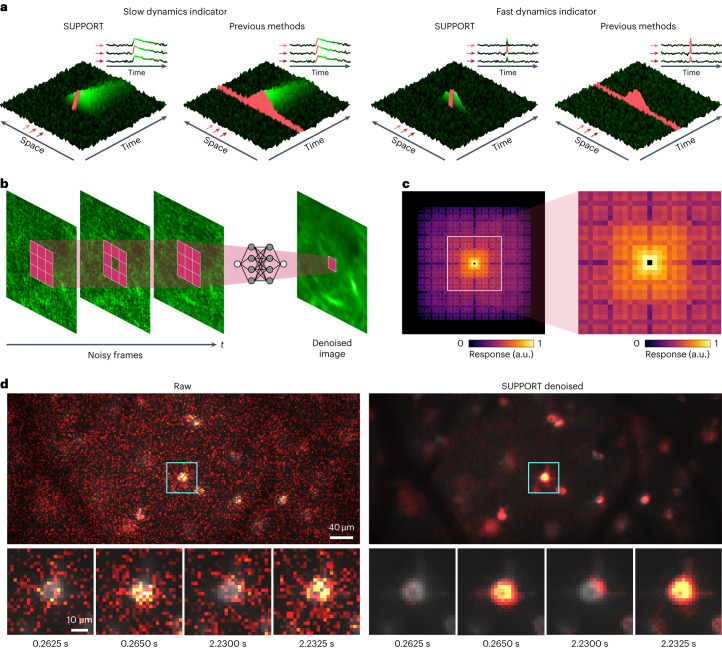
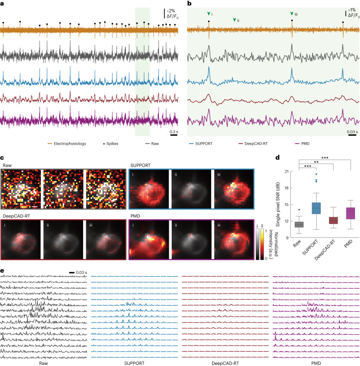
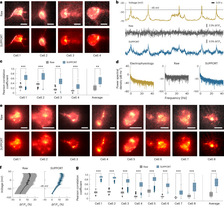
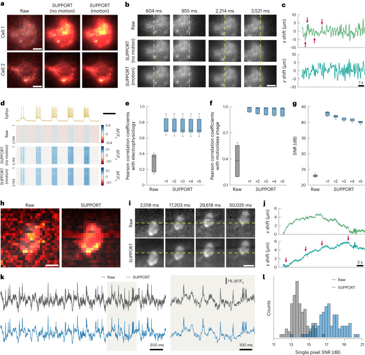
Here we report SUPPORT (statistically unbiased prediction utilizing spatiotemporal information in imaging data), a self-supervised learning method for removing Poisson-Gaussian noise in voltage imaging data. SUPPORT is based on the insight that a pixel value in voltage imaging data is highly dependent on its spatiotemporal neighboring pixels, even when its temporally adjacent frames alone do not provide useful information for statistical prediction. Such dependency is captured and used by a convolutional neural network with a spatiotemporal blind spot to accurately denoise voltage imaging data in which the existence of the action potential in a time frame cannot be inferred by the information in other frames. Through simulations and experiments, we show that SUPPORT enables precise denoising of voltage imaging data and other types of microscopy image while preserving the underlying dynamics within the scene.

Fig. 1. SUPPORT can be applied to functional imaging data with a fast dynamics indicator.

a, SUPPORT’s self-supervised learning scheme and previous methods that exploit temporally adjacent frames for denoising functional imaging data with slow and fast dynamics indicators. Functional imaging data are represented by green and red surfaces, which indicate the receptive field and prediction target area, respectively. b, Noisy frames are fed into the SUPPORT network and output the denoised image. Red tiles indicate the receptive field of the SUPPORT network, which uses spatially adjacent pixels in the same frame. c, Impulse response of the SUPPORT network on the current frame. The magnified view is presented on the right side. Response value of the center pixel is 0, which forces the network to predict the center pixel without using it. d, In vivo population voltage imaging data. The left shows the raw data and the right shows the SUPPORT-denoised data. Baseline and activity components are decomposed from raw data and SUPPORT-denoised data. The baseline component with gray colormap and activity component with hot colormap are overlaid. Magnified views of the boxed regions are presented below at the time points near spikes. Consecutive frames of two spikes (t = 0.2650 and 2.2325 s).

Fig. 2. Performance validation on simulated data.

a, Synthetic population voltage imaging data. From left to right are the clean, noisy, SUPPORT, DeepCAD-RT and PMD denoised data. Baseline and activity components are decomposed from the data. The baseline component with a gray colormap and activity component with a hot colormap are overlaid. Magnified views of the boxed regions are presented underneath with the consecutive frames of the spiking event (t = 0.222 s). Scale bar, 40 μm. b, PSNR of the baseline-corrected data before and after denoising data with different spike widths. Clean data were used as the ground truth for PSNR calculation. c, The left shows a box-and-whisker plot showing Pearson correlation coefficients before and after denoising data with different spike widths. The right shows a line chart showing average Pearson correlation coefficient before and after denoising data with different spike widths. Two-sided one-way analysis of variance with Tukey–Kramer post hoc test was used. n = 116 for each test, which represents the number of neurons (NS, not significant, *P < 0.1, **P < 0.01, ***P < 0.001). d, Single-pixel fluorescence traces extracted from baseline-corrected data. From top to bottom: clean, noisy, SUPPORT, DeepCAD-RT and PMD denoised data. The left shows each single-pixel trace occupies each row. The right shows three representative single-pixel traces visualized with different colors. e, Single cell fluorescence traces near spiking event extracted from baseline-corrected data. From top to bottom: clean, noisy, SUPPORT, DeepCAD-RT and PMD denoised data. From left to right: changing spike widths of 1, 3, 5, 7 and 9 ms. Source data

Fig. 3. Denoising single-neuron voltage imaging data.

a, Simultaneous electrophysiological recording and voltage imaging data. From top to bottom: electrophysiological recording, raw, SUPPORT, DeepCAD-RT and PMD denoised data. Detected spikes from electrophysiological recordings are marked with black dots. Traces from voltage imaging data were extracted using a manually drawn ROI. b, Enlarged view of the green region in a. c, Three representative frames indicated on b with green arrows for raw and denoised data. Baseline and activity components are decomposed from raw data and denoised data. The baseline component with a gray colormap and the activity component with a hot colormap are overlaid. Scale bar, 1 μm. d, Box-and-whisker plot showing the SNR for the pixels inside the cell region from raw and denoised data. From left to right: raw, SUPPORT, DeepCAD-RT and PMD denoised data. Two-sided one-way analysis of variance with Tukey–Kramer post hoc test was used. n = 70 for each test, which represents the number of pixels (*P < 0.1, **P < 0.01, ***P < 0.001). e, Spatiotemporal diagram showing the voltage transients of each 2 × 2 binned pixel with a small temporal region centered at time point i on b. From left to right: raw, SUPPORT, DeepCAD-RT and PMD denoised data. Source data

Fig. 4. Recovering subthreshold activity in voltage imaging data.

a, Raw and SUPPORT-denoised images of four neurons in mouse cortex layer 1 expressing Voltron1 are shown after baseline correction. Scale bars, 5 μm. b, Electrophysiological recording and single-pixel traces extracted from raw and SUPPORT-denoised data. Spike regions are detected from electrophysiological recording data and excluded in subthreshold analysis. c, The left shows box-and-whisker plots showing Pearson correlation coefficient between electrophysiological recording and single-pixel fluorescence traces in subthreshold region. The right shows box-and-whisker plots showing average Pearson correlation coefficients before and after denoising. A two-sided paired-sample t-test was used: cell 1, n = 1,842; cell 2, n = 675; cell 3, n = 2,610; cell 4, n = 506 and average, m = 4, where n represents the number of pixels and m represents the number of cells. d, Power spectral density of electrophysiological recording and single-pixel fluorescence traces of raw and denoised data. e, Raw and SUPPORT-denoised images of eight neurons in the brain slice from mouse cortex L2/3 expressing QuasAr6a are shown after baseline correction. Scale bars, 10 μm. f, Relationship between transmembrane potential and dF/F₀. Average and standard deviation of dF/F₀ values are calculated for corresponding voltage values. Average points are drawn as solid lines and areas between average + standard deviation and average-standard deviation are filled. g, The left shows box-and-whisker plots showing Pearson correlation coefficient between electrophysiological recording and single-pixel fluorescence traces in subthreshold region. The right shows box-and-whisker plots showing average Pearson correlation coefficients before and after denoising. A two-sided paired-sample t-test was used: cell 1, n = 3,289; cell 2, n = 3,157; cell 3, n = 3,458; cell 4, n = 3,516; cell 5, n = 2,214; cell 6, n = 599; cell 7, n = 1,240; cell 8, n = 427 and average, m = 8, where n represents the number of pixels and m represents the number of cells (**P < 0.01, ***P < 0.001). Source data

Fig. 5. Denoising population voltage imaging data.

a, Images after baseline correction from mouse dataset. The top shows the baseline-corrected raw data. The bottom shows the baseline-corrected SUPPORT-denoised data. Boundaries of two ROI are drawn with cyan lines. Scale bar, 40 μm. b, Distribution of the SNR for all pixels from raw and SUPPORT-denoised data after baseline correction, n = 65,536. c, Traces from raw and SUPPORT-denoised data extracted from two ROI in a. Traces for the smaller temporal region are plotted on the right. The enlarged temporal region is colored blue and brown. d, Images from the zebrafish dataset. Baseline and activity components are decomposed from raw data and SUPPORT-denoised data. The baseline component with a gray colormap and the activity component with a hot colormap are overlaid. Boundaries of 20 ROI are drawn with cyan lines. The top shows raw data. The bottom shows SUPPORT-denoised data. Scale bar, 20 μm. e, Distribution of SNR for pixels inside the ROI from raw and SUPPORT-denoised data, n = 5,722. f, Traces for 20 ROI from raw and SUPPORT-denoised data. The left shows raw data. The right shows SUPPORT-denoised data. g, Enlarged view of traces from colored regions in f is plotted. Traces from raw data are overlaid with a gray color and denoised data are overlaid with corresponding color in f.

Fig. 6. Denoising voltage imaging data with motion.

a, Representative frames of raw video and SUPPORT-denoised videos without and with motion after baseline correction. Motion was synthetically applied to the images of neurons in mouse cortex L2/3 expressing QuasAr6a, simultaneously recorded with electrophysiology. Scale bars, 5 μm. b, Representative frames of a spatially expanded view of cell 1 in a at the timings indicated by red arrows in c. From left to right: frames at 604, 955, 2,214 and 3,521 ms. From top to bottom: raw video, SUPPORT-denoised video without motion and SUPPORT-denoised video with motion. Scale bar, 5 μm. c, Line plot showing the x and y direction motions in the micrometer scale. d, Electrophysiology trace and single-pixel fluorescence traces extracted from the videos. From top to bottom: electrophysiology, raw video, SUPPORT-denoised video without motion and SUPPORT-denoised video with motion. Scale bar, 500 ms. e, Box-and-whisker plot showing Pearson correlation coefficients between fluorescence traces and electrophysiology, before and after denoising. ×5 indicates a five times higher motion compared to ×1. n = 5, which represents the number of cells. f, Box-and-whisker plot showing Pearson correlation coefficients between ground-truth image (SUPPORT-denoised image without motion) and images with motion before and after denoising. n = 5, which represents the number of cells. g, Box-and-whisker plot showing SNR acquired by comparing ground-truth image and images with motion before and after denoising. n = 5, which represents the number of cells. h, Representative frames of raw video and SUPPORT-denoised videos after baseline correction. The images show a neuron expressing SomArchon in the hippocampus of an awake mouse. Scale bar, 3 μm. i, Representative frames in h at the timings indicated by red arrows in j. From left to right: frames at 2,018, 17,203, 29,618 and 50,025 ms. Scale bar, 5 μm. j, Line plot showing x and y directional motions in the micrometer scale. k, Traces extracted from a single cell in raw video and SUPPORT-denoised video. Temporally expanded traces from the brown area on the left are shown on the right. l, Histogram of SNR from the raw video and SUPPORT-denoised video. Source data

Extended Data Fig. 1. SUPPORT denoises freely moving Caenorhabditis elegans imaging data.

a, Images of freely moving C. elegans. From left to right: Noisy, SUPPORT, DeepCAD-RT, and PMD denoised data. Inset shows the intensity profile along the dashed line. Magnified views of the boxed regions are presented underneath. b, Pixel-wise difference between denoised data and noisy data. Squared norm of Fourier transform of each difference are shown in the lower images. Inset shows the logarithm of the squared norm of Fourier transform against the distance to the origin. c, Magnified views of the red boxed region in a at consecutive neighboring time points. Magenta lines were set on the left side of the brightest neuron in the noisy data. From top to bottom: Noisy, SUPPORT, DeepCAD-RT, and PMD denoised data. d, Noisy volume and denoised volume are depth coded and presented. Magnified views of the boxed regions are presented on the right.

Extended Data Fig. 2. SUPPORT denoises volumetric structural imaging data.

a, Representative axial slice from low-SNR, SUPPORT-denoised, high-SNR volumes of Penicillium. b, Magnified views of the yellow boxed region in a at multiple axial locations. Axial location of a corresponds to 3.37 μm. c, Box-and-whisker plot showing Pearson correlation coefficient and signal-to-noise ratio for axial slices. A two-sided paired-sample t-test is used, N = 381, which represents the number of planes along the z-axis (***: p-value < 0.001). d, Intensity profiles of the cyan dashed line in a. e, Example frame of bone of a mouse embryo after expansion for the raw data (top) and denoised image using SUPPORT (bottom). f, Raw (top) and denoised image (bottom) of intestine of a mouse embryo. e-f, Length scales are presented in pre-expansion dimensions. Source data

References

1. Calarco JA, Samuel AD. Imaging whole nervous systems: insights into behavior from worms to fish. Nat. Methods. 2019;16:14–15. doi: 10.1038/s41592-018-0276-8. - DOI - PMC - PubMed
1. Resendez SL, et al. Visualization of cortical, subcortical and deep brain neural circuit dynamics during naturalistic mammalian behavior with head-mounted microscopes and chronically implanted lenses. Nat. Protoc. 2016;11:566–597. doi: 10.1038/nprot.2016.021. - DOI - PMC - PubMed
1. Streich L, et al. High-resolution structural and functional deep brain imaging using adaptive optics three-photon microscopy. Nat. Methods. 2021;18:1253–1258. doi: 10.1038/s41592-021-01257-6. - DOI - PMC - PubMed
1. Chen BC, et al. Lattice light-sheet microscopy: imaging molecules to embryos at high spatiotemporal resolution. Science. 2014;346:1257998. doi: 10.1126/science.1257998. - DOI - PMC - PubMed
1. Yoon YG, et al. Sparse decomposition light-field microscopy for high speed imaging of neuronal activity. Optica. 2020;7:1457–1468. doi: 10.1364/OPTICA.392805. - DOI
Publication types