Identification of mobile genetic elements with geNomad

Abstract

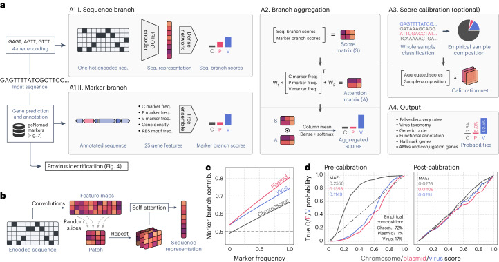
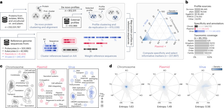
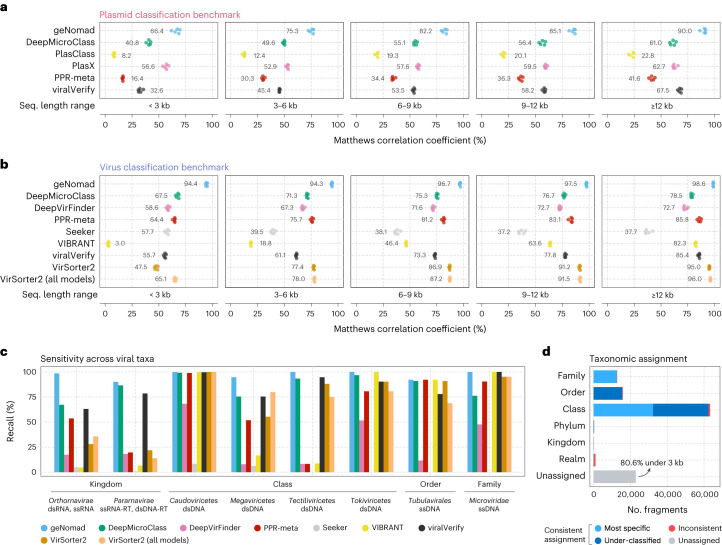
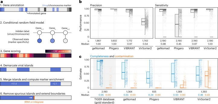
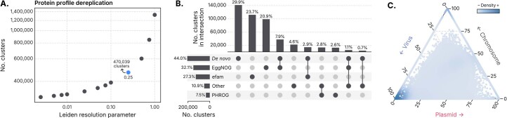
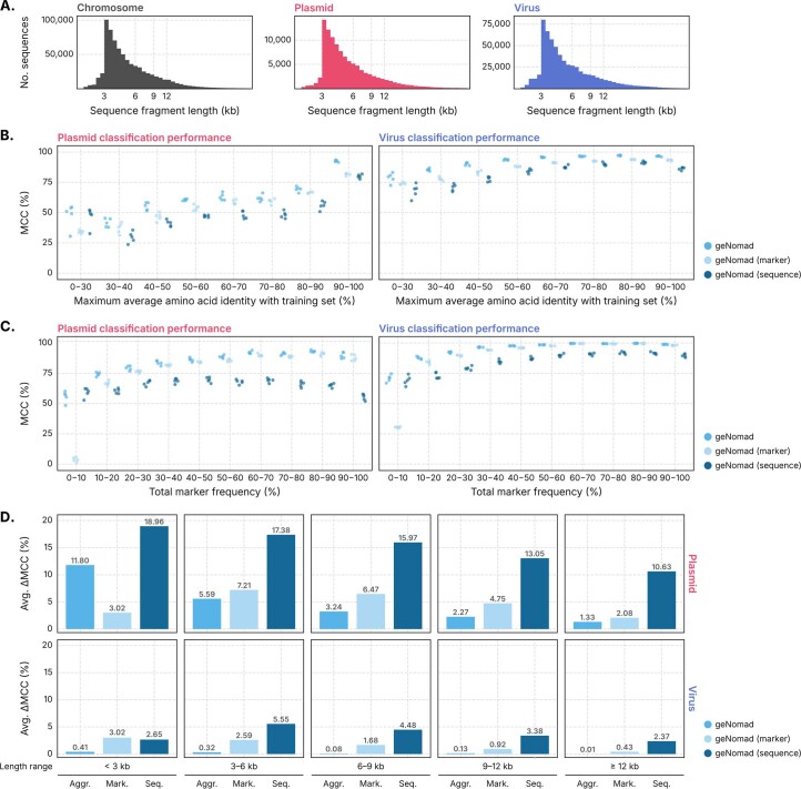
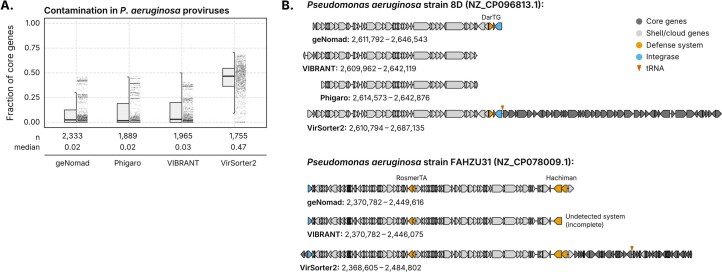
Identifying and characterizing mobile genetic elements in sequencing data is essential for understanding their diversity, ecology, biotechnological applications and impact on public health. Here we introduce geNomad, a classification and annotation framework that combines information from gene content and a deep neural network to identify sequences of plasmids and viruses. geNomad uses a dataset of more than 200,000 marker protein profiles to provide functional gene annotation and taxonomic assignment of viral genomes. Using a conditional random field model, geNomad also detects proviruses integrated into host genomes with high precision. In benchmarks, geNomad achieved high classification performance for diverse plasmids and viruses (Matthews correlation coefficient of 77.8% and 95.3%, respectively), substantially outperforming other tools. Leveraging geNomad's speed and scalability, we processed over 2.7 trillion base pairs of sequencing data, leading to the discovery of millions of viruses and plasmids that are available through the IMG/VR and IMG/PR databases. geNomad is available at https://portal.nersc.gov/genomad .

Fig. 1. A hybrid framework for identifying and annotating plasmids and viruses.

a, geNomad processes user-provided nucleotide sequences through two branches. In the sequence branch, the inputs are one-hot encoded fed to an IGLOO neural network, which scores inputs based on the detection of non-local sequence motifs (A1 I). In the marker branch, proteins encoded by the input sequences are annotated using markers that are specific to chromosomes, plasmids or viruses (A1 II). A set of numerical features is then extracted from the annotated proteins and fed to a tree ensemble model, which scores the inputs based on their marker content. Next, the scores provided by both branches are aggregated by weighing the contribution of each branch based on the frequency of markers in the sequence (A2). Aggregated scores can then be calibrated to approximate probabilities in a process that leverages the sample composition inferred from the classification of sequences from the same batch (A3). Lastly, classification results are summarized and presented together with additional data, such as virus taxonomy, gene function and the inferred genetic code (A4). b, The sequence branch is based on the IGLOO architecture, which uses convolutions to produce a feature map from a one-hot encoded input. Patches encoding non-local relationships within the sequence are then generated by slicing the feature map. Lastly, these patches are used as an attention matrix to produce a sequence representation from the feature map. c, The relative contribution of the marker branch (y axis, quantified using SHAP) increases as the marker frequency (fraction of genes assigned to a marker) in the sequence increases. d, Calibration curves of pre-calibration (left) and post-calibration (right) scores, showing that sample composition can be used to map classification scores to actual probabilities. The x axis represents scores averaged across multiple bins; the y axis represents the fraction of positives in each bin; the 45° dashed line represents a perfect calibration scenario. freq., frequency; MAE, mean absolute error of the scores relative to the true probabilities.

Fig. 2. Generating of a dataset of protein profiles with abundant metadata for sequence classification and protein annotation.

a, Protein sequences from genomes and metagenomes were clustered and aligned to produce de novo protein profiles. De novo profiles and profiles obtained from public databases were then clustered, and cluster representatives were selected to reduce redundancy. In parallel, reference chromosome, plasmid and virus sequences were clustered into RCs. Sequences were then weighed in such a way that the sum of the weights within each RC was constant. Representative protein profiles were mapped to reference sequences, and chromosome-, plasmid- and virus-specificity metrics were computed for each profile based on the weighed number of hits to sequences of each class. Markers that were highly specific to one of the three classes were then selected. The position of each selected marker (circles) in the ternary plot is determined by its specificity, and the colors represent the marker density in a region. b, Bar plots showing: the sources of the selected profiles (upper plot); the total number of markers (light shades) and the number of functionally annotated markers (dark shades) for each class (middle plot); and the fraction of ICTV taxa covered by the taxonomically informative markers at each rank. c, Multidimensional scaling of semantic similarities of the GO terms enriched in chromosome (left), plasmid (center) and virus (right) markers. Labels of related terms were aggregated for clarity. Semantic similarities were computed with REVIGO. d, RadViz visualizations of the relative frequencies of geNomad markers across distinct ecosystems. Each marker is represented by a circle, and the colors depict the marker density within a region. The position of the markers in the plot is determined by their frequency in each environment. Markers close to the center of the plot were found in similar frequencies across all ecosystems. Median entropies of the ecosystem distributions are shown below the plots. AF, aquatic (freshwater); AM, aquatic (marine); AO, aquatic (other); EN, engineered; HA, host-associated (animals); HO, host-associated (other); HP, host-associated (plants); TO, terrestrial (other); TS, terrestrial (soil).

Fig. 3. geNomad accurately identifies viruses and plasmids and allows taxonomic assignment of viral genomes.

a,b, Classification performance of multiple plasmid (a) and virus (b) identification tools across sequence fragments of varying length. Performance was measured using the MCC. For each sequence range interval, tools were evaluated with five different test sets, each containing the sequences of one RC. Colored circles represent the performances measured in each test set. Mean values are shown next to the circles. c, Sensitivity of virus identification tools across major viral taxa at different ranks. The score cutoff of each tool was determined so that the FDR was approximately 5%. d, Virus taxonomic assignment performance. Bar lengths represent the number of sequence fragments assigned at a given taxonomic rank. Light blue represents sequences that were correctly assigned to their most specific rank (up to the family level); dark blue represents fragments that were assigned to the correct lineage but to a rank that is above its most specific rank; red represents sequences that were assigned to the wrong lineage; and the gray bar represents sequences that were assigned to any taxon.

Fig. 4. geNomad uses marker information to demarcate provirus boundaries.

a, Provirus identification starts by annotating the genes within a sequence with geNomad markers, which store information of how specific they are to hosts or viruses. These specificity values are then fed to a CRF model, which will score each gene using information from the markers in its surroundings. A score cutoff is used to demarcate viral islands, and islands that are close together are merged. Islands with few viral markers are discarded, and the boundaries of the remaining islands are extended up until nearby tRNAs or integrases. b, Distributions of the precision and sensitivity of multiple provirus identification tools, measured at the gene level for each provirus. Proviruses from the TIGER database were used as the ground truth for this benchmark. c, Completeness and contamination estimates of demarcated proviral regions that did not overlap with proviruses in the TIGER database. Estimates for TIGER proviruses are shown with a gray background as a reference. Box plots show the median (middle line), interquartile range (box boundaries) and 1.5 times the interquartile range (whiskers).

Fig. 5. geNomad allows the discovery of RNA viruses and giant viruses in environmental sequencing data.

a, Histograms showing the geNomad score distribution of three groups of scaffolds of the Sand Creek Marshes metatranscriptomes: scaffolds that binned with RdRP-encoding sequences (top row, in green); scaffolds that contain the RdRP gene (middle row, in blue); and the remaining scaffolds (bottom row, in orange). The median geNomad score and the fraction of scaffolds classified as viral are indicated for each group. b, Genome maps of selected sequences that were classified as viral by geNomad. Two pairs of co-occurring Orthornavirae scaffolds are represented (Marnaviridae and Cystoviridae bins). Genes targeted by geNomad markers are colored, and genes that do not match any marker are shown in gray. Rows and colors match those of a. c, Number of scaffolds assigned to Nucleocytoviricota orders across multiple ecosystems (left bar plot). Sequences were identified by geNomad in a large-scale survey of metagenomes of diverse ecosystems. Only scaffolds that are at least 50 kb long or more were evaluated. Bar colors represent the ecosystem types where the sequences were identified. The phylogenetic diversity (PD) fold change is shown on the right bar plot. PD fold change values correspond to the ratio between the total PD of trees reconstructed with and without geNomad-identified giant viruses. d, Maximum likelihood phylogenetic tree of soil giant viruses identified with geNomad (brown tree tips). Reference sequences from GenBank and from a previous metagenomic survey (GVMAGs) were included, and the ones that were sequenced from soil samples are indicated with turquoise tree tips. Tree tips that are not colored represent representative genomes sequenced from samples obtained from other ecosystems. The ranges corresponding to different Nucleocytoviricota orders are represented using distinct colors.

Extended Data Fig. 1. Global sequence representations generated by the IGLOO encoder are used for sequence classification.

(a) The IGLOO encoder applies 128 independent convolutions to the one-hot-encoded sequence to create a feature map, from which four random slices are taken and concatenated to generate patches that encode long-distance relationships within the sequence. (b) A total of 2,100 patches are used to weight different parts of the feature map in a transformer-like self-attention mechanism that results in a high-dimensional sequence representation. The encoder was trained using a supervised contrastive loss function, which optimizes the separation of the three classes (chromosome, plasmid, and virus) in the embedding space. (c) To classify sequences, the sequence representations generated by the IGLOO encoder are fed to a dense neural network trained with focal loss to account for class imbalance.

Extended Data Fig. 2. Sample composition can be leveraged to calibrate classification scores to approximate probabilities.

(a) The false positive rates of a set of classifications depend on the sample’s underlying composition. In typical metagenomes, where cellular sequences outnumber viral sequences, the fraction of false positives within scaffolds classified as viral is higher than in a virome. (b) The mean absolute error (MAE) of the score calibration model (y-axis) is highly dependent on the number of sequences in the sample (x-axis), as larger samples will result in more accurate estimates of the underlying sample composition. (c) The calibration model tends to increase the scores of a given class when it is abundant in the sample and reduce the scores when the class is rare. (d) The relative frequency of a given class in the sample (x-axis) contributes positively to the model output (y-axis, quantified using SHAP) when that class is abundant in the sample and negatively when the class is rare. (e) The pre-calibration score of a given class in the sample (x-axis) contributes positively to the model output (y-axis, quantified using SHAP) when the initial score is high and negatively when the initial score is low.

Extended Data Fig. 3. Assigning viral taxa using geNomad’s markers.

(a) To assign viral sequences to specific taxa, geNomad utilizes a best-hit approach to initially assign the genes encoded by these sequences to markers. (b) Each gene is subsequently classified based on the taxonomic lineage of the assigned marker. Different genes within the sequence might be assigned to different lineages. (c) To establish a single sequence-level taxonomy, geNomad aggregates the lineages of all the markers using a weighted majority vote approach. This approach determines the support for each taxon at each taxonomic rank by summing the bitscores of all genes assigned to that taxon. The sequence is then assigned to the most specific taxon that is supported by at least 50% of the total bitscore of the sequence.

Extended Data Fig. 4. geNomad’s marker dataset was built by gathering dereplicated protein profiles from several sources and measuring their specificity to chromosomes, plasmids, and viruses.

(a) Number of protein profile clusters obtained by varying the clustering granularity (Leiden’s resolution parameter). The value chosen for dereplication (0.25) is indicated in blue. (b) UpSet plot showing the overlap of different protein profile datasets in the dereplication process. The overlap between a given pair of datasets was measured as the number of protein profile clusters that contained profiles from both. (c) Ternary plot showing the specificity of protein profiles (circles) prior to dereplication (n = 470,039). Colors represent the marker density in a region of the plot.

Extended Data Fig. 5. geNomad can detect plasmids and viruses with low identity to the training data even if they encode few or no markers.

(a) Length distributions of the sequence fragments used to train geNomad and to evaluate classification performance of multiple tools. Sequence length (x-axis) is represented in log scale. (b) geNomad’s classification performance on plasmids (left) and viruses (right) with varying degrees of similarity to sequences in the train data (bins in the x-axis). Similarity to the train data was assessed by computing average amino acid identities to the sequences in the train data. (c) geNomad’s classification performance on plasmids (left) and viruses (right) with varying marker frequency (fraction of genes assigned to a geNomad marker). For each interval, performance was measured across five pairs of train/test sets (leave-one-group-out strategy). (d) Score calibration improves classification performance for both plasmids and viruses across all length ranges. Classification performance was measured using the Matthews correlation coefficient (MCC).

Extended Data Fig. 6. geNomad outperforms other tools in identifying proviruses in the Pseudomonas aeruginosa pangenome.

(a) Distribution of the contamination estimates of multiple provirus-identification tools, measured at the gene-level for each provirus. Contamination was measured as the number of core genes, as determined by PPanGGOLiN, in the provirus. The number of detected provirus and the median contamination of each tool are displayed below the graph. Box plots show the median (middle line), interquartile range (box boundaries), and 1.5 times the interquartile range (whiskers). (b) Defense system-encoding proviral regions demarcated with multiple tools in P. aeruginosa genomes. Shell and cloud genes are shown in light grey and core genes (putative contamination) are shown in dark gray. Genes that are part of defense systems are in orange. Integrase genes are in blue. tRNA loci are indicated by red arrows. GenBank accessions are shown within parenthesis. Phigaro did not detect any provirus within the 2,370,782–2,449,616 bp region in the NZ_CP078009.1 sequence.

References

1. Rodríguez-Beltrán, J., DelaFuente, J., León-Sampedro, R., MacLean, R. C. & San Millán, Á.Beyond horizontal gene transfer: the role of plasmids in bacterial evolution. Nat. Rev. Microbiol.19, 347–359 (2021). 10.1038/s41579-020-00497-1 - DOI - PubMed
1. Suttle, C. A. Viruses in the sea. Nature437, 356–361 (2005). 10.1038/nature04160 - DOI - PubMed
1. Ochman, H., Lawrence, J. G. & Groisman, E. A. Lateral gene transfer and the nature of bacterial innovation. Nature405, 299–304 (2000). 10.1038/35012500 - DOI - PubMed
1. de la Cruz, F. & Davies, J. Horizontal gene transfer and the origin of species: lessons from bacteria. Trends Microbiol.8, 128–133 (2000). 10.1016/S0966-842X(00)01703-0 - DOI - PubMed
1. Eraslan, G., Avsec, Ž., Gagneur, J. & Theis, F. J. Deep learning: new computational modelling techniques for genomics. Nat. Rev. Genet.20, 389–403 (2019). 10.1038/s41576-019-0122-6 - DOI - PubMed