Jupiter Science Enabled by ESA's Jupiter Icy Moons Explorer

Abstract

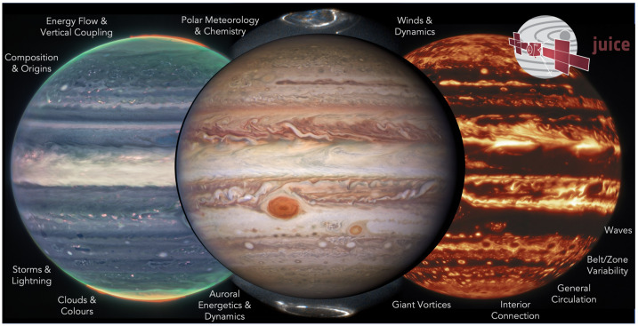
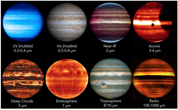
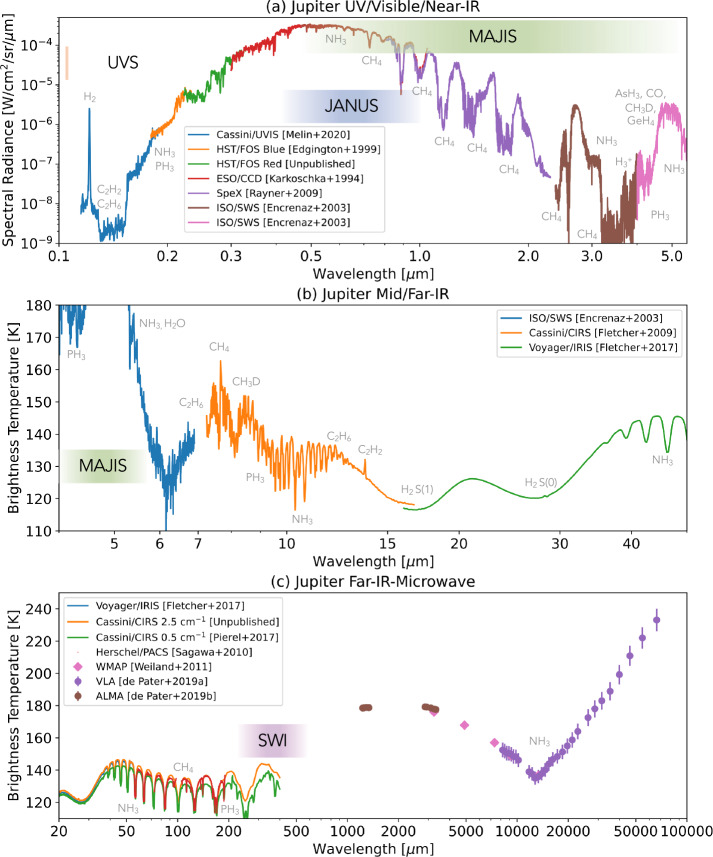
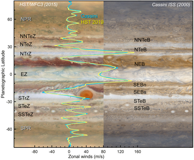
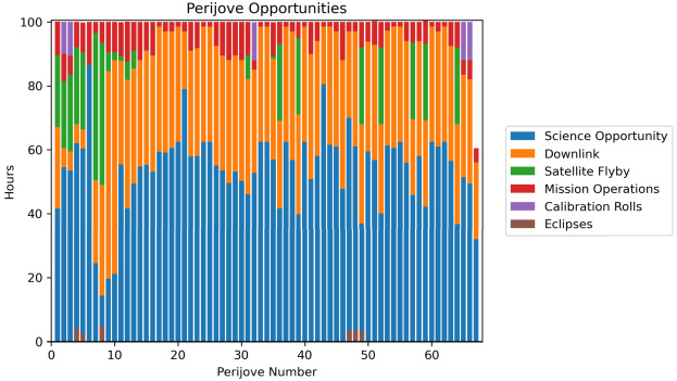
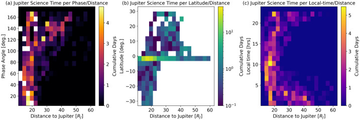
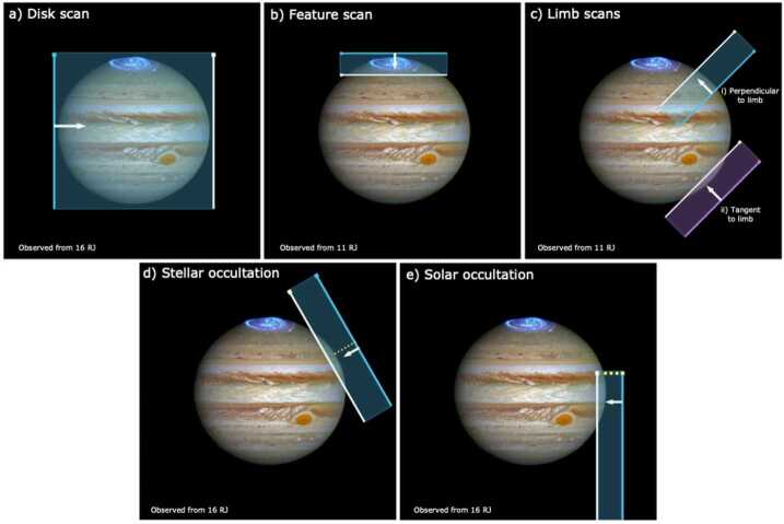
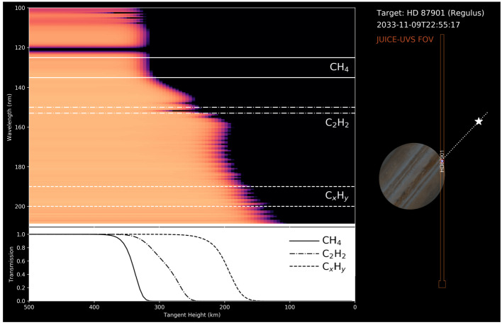
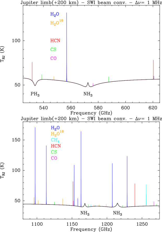
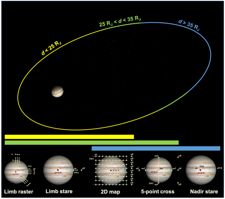
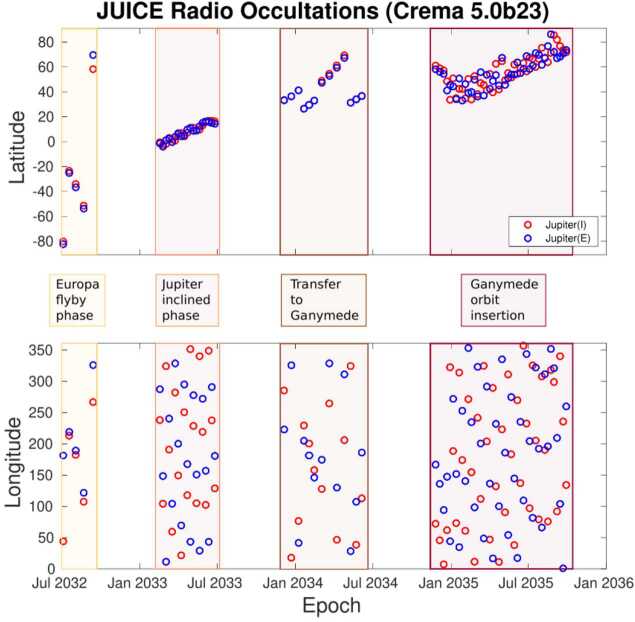
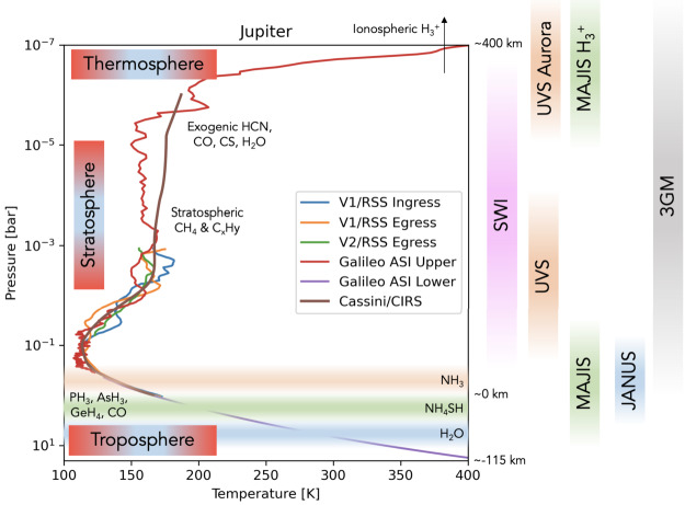
ESA's Jupiter Icy Moons Explorer (JUICE) will provide a detailed investigation of the Jovian system in the 2030s, combining a suite of state-of-the-art instruments with an orbital tour tailored to maximise observing opportunities. We review the Jupiter science enabled by the JUICE mission, building on the legacy of discoveries from the Galileo, Cassini, and Juno missions, alongside ground- and space-based observatories. We focus on remote sensing of the climate, meteorology, and chemistry of the atmosphere and auroras from the cloud-forming weather layer, through the upper troposphere, into the stratosphere and ionosphere. The Jupiter orbital tour provides a wealth of opportunities for atmospheric and auroral science: global perspectives with its near-equatorial and inclined phases, sampling all phase angles from dayside to nightside, and investigating phenomena evolving on timescales from minutes to months. The remote sensing payload spans far-UV spectroscopy (50-210 nm), visible imaging (340-1080 nm), visible/near-infrared spectroscopy (0.49-5.56 μm), and sub-millimetre sounding (near 530-625 GHz and 1067-1275 GHz). This is coupled to radio, stellar, and solar occultation opportunities to explore the atmosphere at high vertical resolution; and radio and plasma wave measurements of electric discharges in the Jovian atmosphere and auroras. Cross-disciplinary scientific investigations enable JUICE to explore coupling processes in giant planet atmospheres, to show how the atmosphere is connected to (i) the deep circulation and composition of the hydrogen-dominated interior; and (ii) to the currents and charged particle environments of the external magnetosphere. JUICE will provide a comprehensive characterisation of the atmosphere and auroras of this archetypal giant planet.

Keywords: Atmospheres; Auroras; Chemistry; Dynamics; JUICE; Jupiter.

Fig. 1

Summary of the Jupiter science enabled by the JUICE mission. Images show Jupiter in visible light from Hubble (centre, Credit: NASA, ESA, NOIRLab, NSF, AURA, M.H. Wong and I. de Pater et al.), near-infrared from JWST (left, using 3.6 μm (red), 2.12 μm (yellow-green), and 1.5 μm (cyan); credit: NASA, ESA, CSA, Jupiter ERS Team; image processing by Judy Schmidt), and in the 5-μm window (right, credit: Gemini Observatory, NOIRLab, NSF, AURA, M.H. Wong et al.), where clouds from the visible/near-IR images (sensing $\sim 0.1-3$ bars) appear in silhouette against the thermal background from the 4-6 bar region. Auroral emissions from H₃⁺ can be seen in the JWST image, and in the UV in Hubble observations (centre-top and centre-bottom, credit: NASA, ESA. J. Clarke)

Fig. 2

Multi-wavelength remote sensing of Jupiter provides access to both reflected sunlight (UV to near-IR) and thermal emission (mid-IR to radio). These false-colour images demonstrate the appearance of the atmosphere at different wavelengths. JUICE UVS will measure scattered sunlight from upper-tropospheric aerosols. JANUS and MAJIS observations (below approximately 3 μm) sense clouds, chromophores and winds in the cloud decks using both the continuum and strong CH₄ absorption bands (Hueso et al. ; Grassi et al. 2020). MAJIS will be able to observe H₃⁺ emission from Jupiter’s ionosphere and auroras between 3-4 μm (VLT/ISAAC observations, Credit: ESO), as well as thermal emission from the deep cloud-forming layers (4-6 bars) near 5 μm (Gemini/NIRI observation, Wong et al. 2020). Although JUICE lacks mid-IR capabilities (VLT/VISIR observations sensing the upper troposphere at 0.1-0.5 bars, and stratosphere at 1-10 mbar, Fletcher et al. 2017a) and radio-wavelength capabilities (VLA observations, de Pater et al. 2016), sub-millimetre sounding by SWI will probe the stratospheric temperatures and winds. The approximate sensitivity of the JUICE instruments to different altitudes is shown in Fig. 26

Fig. 3

Overview of Jupiter’s reflected ($\lambda <4$ μm) and thermal emission ($\lambda >4$ μm) spectra, with key molecular features labelled, and the approximate ranges covered by UVS, JANUS, MAJIS and SWI. UV, visible, and near-IR spectra in (a) were created from a low-latitude spectrum from Cassini/UVIS (Melin et al. 2020); Hubble FOS spectra at $6-{20}^{\circ }$N acquired in November 1992 with the blue and red detectors (Edgington et al. 1999); disc-averaged measurements from the European Southern Observatory (Karkoschka 1994) converted from albedo to spectral radiance assuming the solar spectrum of (Meftah et al. 2018); disc-averaged measurements from IRTF SpeX instrument (Rayner et al. 2009) approximately scaled to match adjacent datasets; and disc-averaged ISO/SWS measurements from Encrenaz (2003). Mid- and far-IR spectra in (b) were from ISO/SWS, plus low-latitudes averages from Cassini/CIRS (Fletcher et al. 2009) and Voyager-1/IRIS (Fletcher et al. 2017b). Far-IR to microwave spectra in (c) were from averaged Cassini/CIRS spectra (Pierel et al. 2017), Herschel/PACS observations (Sagawa et al. 2010); and disc-averaged brightnesses from WMAP and ALMA in the millimetre (Weiland et al. ; de Pater et al. 2019a) and VLA in the centimetre (de Pater et al. 2019b)

Fig. 4

Jupiter belts and zones, defined by the zonal winds, compared to contrasts in colour and reflectivity. White zones and reddish belts alternate in latitude following the anticyclonic and cyclonic shear of the zonal jets. The locations and overall characteristics of the jets and the bands are stable in time, but the magnitude of the winds and the intensity of the belt/zone colors are variable. Zonal winds in this figure come from Cassini in 2000 (Porco et al. 2003) and from Hubble images from 2019 following an equivalent analysis to that presented in Hueso et al. (2017). The conventional names of zones (left) and belts (right) are given. The HST background on the left comes from the HST/OPAL program and is available at http://dx.doi.org/10.17909/T9G593. The Cassini map is available at NASA photojournal as image PIA02864

Fig. 5

Vertical structure of Jupiter’s troposphere and lower stratosphere. Deriving the vertical cloud structure at different locations from JANUS/MAJIS data will require the use of radiative transfer models. Reflected-sunlight observations will be sensitive to levels from $\sim 100$ mbar (in the methane absorption band with JANUS) to at least 2.5 bar (in the IR images from MAJIS) with some contributions from deeper layers (Wong et al. 2023). (a) In a cloudless atmosphere imaging filters from the blue to red wavelengths can penetrate deep in the atmosphere limited by Rayleigh scattering and methane absorptions at specific wavelengths such as in 727 and 890 nm (contribution functions for single wavelengths from Dahl et al. 2021). (b) The nominal cloud structure in Jupiter consists of layers of ammonia, ammonia hydrosulphide and water clouds with approximate cloud bases at around 0.7, 2.5, 5-7 bar, respectively, depending on the local abundance of condensables. The thermochemical calculation shown here assumes 3 times solar abundance of condensables (see Atreya et al. , for details), but the NH₃ abundance below the condensation level is not well mixed, and is now known to vary substantially as a function of altitude and latitude (Li et al. 2017). The upper ammonia cloud limits the penetration depth of visible light. Above the condensate clouds are higher-altitude hazes with varied properties in different Jupiter regions that can be sampled with a combination of methane band images and observations in near-IR wavelengths. (c) The real cloud structure is probably very heterogeneous with locations of deep convection, dry areas and intermediate cloud systems

Fig. 6

Morphology and variety of atmospheric features at different spatial scales (colours are approximate and contrasts have been enhanced for visibility): (a) Jupiter’s Great Red Spot. (b) Turbulent filamentary features at a 52^∘N (white structures) near a dark brown vortex, both showing cyclonic morphologies in their clouds. (c) Convective storm at 31^∘S. (d) Dayside storms with lightning observed at the same location on the nightside. (e) Series of short-scale gravity waves in Jupiter’s cloud at 17^∘N above a series of large dark features at 8^∘N in Jupiter’s North Equatorial Belt. (f) One of the dark projections of the North Equatorial Belt, sometimes known as a 5-μm hotspots. (g) New Horizons observation of small-scale gravity waves in Jupiter’s atmosphere. (h) Galileo observations of Jupiter’s limb in violet and near infrared light at 756 nm. (i) Composite map of Jupiter’s North polar region in polar projection from Junocam observations obtained on different perijoves. (j) combination of visible and near IR observations of Jupiter’s South polar region sampling polar hazes structured as a circumpolar wave. Latitudinal grid is superimposed each 10^∘. Credits and sources: (a) and (b). Junocam images acquired on February 12, 2019 with credits: NASA / JPL-Caltech / SwRI / MSSS / Kevin M. Gill. (c) Excerpt from a Junocam observation obtained on June 2, 2020. (d) Combination of Galileo SSI images obtained on May 4, 1999. NASA / JPL-Caltech. Image (e) is an HST observation from April 1, 2017 from Simon et al. (2018a). Image (f) is a Junocam observation obtained on Sept. 16, 2020. (g) New Horizons views from the MVIC instrument of equatorial waves on Feb. 28, 2007 with credits from NASA/Johns Hopkins University Applied Physics Laboratory/Southwest Research Institute. (h) Galileo December 20, 1996; NASA / JPL-Caltech. (i) Image composite from Junocam images obtained on Feb. 17, April 10, June 2, and July 25 of 2020. NASA/JPL-Caltech/SwRI/MSSS / Gerald Eichstädt, John Rogers. (j) Adapted from Barrado-Izagirre et al. (2008)

Fig. 7

Jupiter’s stratospheric equatorial oscillation was initially discovered from thermal infrared observations similar to those shown in the upper panel (adapted from Antuñano et al. 2021). It is characterised by vertically alternating temperature extrema that descend with time. At a given pressure level (the 3, 6.4, and 13.5 mbar levels are indicated with horizontal dashed lines), positive maxima occur approximately every 4.5 years. Over the years, this oscillation has shown some variability in its periodicity as demonstrated by Giles et al. (2020a) (left panel). The oscillation is not only temporal, but also spatial, as demonstrated on the right panel by the vertically stacked prograde and retrograde jets at the equator (adapted from Benmahi et al. 2021)

Fig. 8

Example auroral images obtained from Jovian orbit at three wavelengths, at different epochs and orientations, with some key features labelled. Lines of System-III longitude and latitude are shown on each. See Fig. 2 of Grodent (2015) for a comprehensive overview of features at UV wavelengths. a) Galileo SSI visible light image of the northern aurora, at a spatial resolution ∼26 km/pix, obtained in November 1997; presented in Fig. 1 of Vasavada et al. (1999), and released as NASA PIA01602 (Credit: NASA/JPL-Caltech). b) Polar projection of May 2017 data from Juno UVS, here showing the southern aurora, presented in detail in Fig. 2 of Bonfond et al. (2021) (Credit: NASA/JPL-Caltech/SwRI/UVS/ULiège). c) Juno JIRAM mosaic map of the southern auroral oval, taken during August 2016. White points are predicted footprint positions indicated by letters I, E, and G for the moons Io, Europa, and Ganymede, respectively. Presented in detail by Mura et al. (2017), Fig. 2 (credit: NASA/JPL-Caltech/SwRI/ASI/INAF/JIRAM)

Fig. 9

Overview of the JUICE orbital tour of Jupiter using Crema 5.0, showing (a) the distance to Jupiter in km; (b) the angular size of Jupiter from JUICE’s vantage point; (c) the sub-spacecraft latitude; and (d) the phase angle (low phase implies dayside, high phase implies nightside). In (a) we show the mean orbital distances of Europa, Ganymede and Callisto for comparison. In (b) we highlight phases 2, 3, 4 and 5 of the tour

Fig. 10

Spatial resolution of JANUS (black line) in the days surrounding Jupiter Orbit Insertion and compared to HST and JWST resolutions (cyan and purple lines, respectively). Phase angle is also plotted (red line)

Fig. 11

Spatial and wind speed resolutions of JANUS and MAJIS as a function of time, based on the Crema 5.0 trajectory and compared to instrumentation on other facilities

Fig. 12

Perijove 12 is used as a generic orbit, from apojove to apojove, to demonstrate the segmentation of the tour. Satellite observations (labelled ‘M’) are prioritised during the $\pm 12$ hours surrounding closest approach. Jupiter atmosphere and auroral science blocks during the $\pm 50$ hour perijove windows (red shading, with specific observations in boxes labelled ‘A’) are interspersed with downlink windows (grey shaded boxes). Atmospheric monitoring (‘D’) is interspersed with dedicated magnetospheric and plasma observations (‘P’) during more distant periods of the orbit. Magnetospheric observations ride along with remote sensing observations during the perijove encounters

Fig. 13

For each perijove, the $\pm 50$-hour perijove windows are subdivided into sub-segments - time available for science observations, time devoted to satellite encounters, telemetry downlink, mission operations (such as navigation images and wheel off-loading), calibration of the magnetometer, and time removed due to Jupiter eclipses

Fig. 14

The cumulative time in days spent in different locations within the Jovian system, showing the phase-angle versus distance to Jupiter in (a); the sub-spacecraft latitude versus distance in (b); and the local time versus distance in (c). Note the logarithmic colour range in (b) to display time spent in the high-inclination phases. Times are only counted if they fall within the Jupiter working group segments

Fig. 15

Examples of JUICE UVS observation techniques at Jupiter. In each example the UVS slit is scaled to its projected size when observing from the distances shown in the bottom left of each panel. The start and end position of the slit is shown, with arrows indicating the direction of slit motion

Fig. 16

Simulation of a Jupiter occultation of bright star Regulus from JUICE UVS. JUICE would hold Regulus fixed in the center of the UVS slit starting a few minutes before ingress until all of its light is blocked by Jupiter. The panels on the left show the ingress occultation light curves spectral resolved (above) and binned over wavelength and labeled by dominant absorber (below). Starting on the left with no light blocked and moving to the right we observe the absorption of the shortest wavelengths first due to H₂ and CH₄ and then followed at longer wavelengths by absorptions by C₂H₂, C₂H₆ and a mix of higher order hydrocarbons (C_xH_y)

Fig. 17

Juno UVS maps from Perijove 3 display the brightness (A) and color ratio (C) of the emissions from Juno’s polar orbit vantage point taken (from supp. in Greathouse et al. 2021). The wire frame model in the center shows the view of Jupiter from JUICE during the high inclination phase and the orientation of the aurora and terminator for the time of the UVS observations (aurora on the night side). Even from a much greater distance, JUICE UVS simulations of the same observation from Juno now displayed in B and D will allow for detailed study of the auroral night side emissions unobservable by Earth-orbiting observatories

Fig. 18

Simulated comparison of Jupiter 5-μm spectra from Juno/JIRAM (blue) and JUICE/MAJIS (orange), based on thermal emission calculations by Grassi et al. (2010). This shows the higher spectral resolution of MAJIS (9.2-10.5 nm) compared to JIRAM (15 nm) in this spectral range, and reveals the longward extension of MAJIS to 5.56 μm. The 5-μm ‘window’ is sculpted by PH₃ absorption on the short-wave side (near 4.3 μm) and NH₃ absorption on the long-wave side (near 5.3 μm), with numerous contributions from minor species (AsH₃, CO, GeH₄, CH₃D and H₂O) as described in the main text

Fig. 19

(Top) Expected coverage of Jupiter’s disk by MAJIS on 2032-Sep-24, near perijove #12. Different colours present the coverage of four cubes acquired at time intervals of 1 h 10 m. (Bottom) Expected coverage of Jupiter’s auroras by MAJIS on 2032-Sep-25, a few hours after perijove #12. Different colours present the coverage of four cubes acquired at time intervals of 46 m

Fig. 20

Example fields-of-view of MAJIS for different observing modes. Each panel presents an individual cube from the set of several that are acquired in close temporal sequence: (top left) A cube from a MAJIS_JUP_DISK_SCAN set; acquisition starts on 2032-Sep-24 at 19:29 UTC, corresponding to the red cube of Fig. 19 (top). (top right) A cube from a MAJIS_JUP_AURORA_SCAN set; acquisition starts on 2032-Sep-25 at 06:51 UTC, corresponding to the red cube of Fig. 19 (bottom). (bottom left) A cube from a MAJIS_JUP_LIMB_SCAN set; acquisition starts on 2032-Sep-25 at 15:24 UTC. (bottom right) Detail of the same MAJIS_JUP_LIMB_SCAN cube

Fig. 21

Jupiter limb spectra in the 600 GHz (top) and 1200 GHz (bottom) bands probed by SWI, with the main observable molecular lines. Spectra are computed at the limb for a tangential height of 200 km above the 1-bar level and are convolved by the instrument beam and to a spectral resolution of 1 MHz

Fig. 22

Example of using the Doppler shift of sub-millimetre spectral lines to determine Jupiter’s stratospheric winds (using ALMA data, Cavalié et al. 2021). The HCN rest frequency is 354.505 GHz (red line), but the observed line is shifted both by the planetary rotation (blue line) and the strong ∼400 m/s westward winds in the south-polar stratosphere (purple line) surrounding regions heated by the Jovian auroras. SWI measurements will use the Doppler shift of several lines to build up a 3D picture of stratospheric winds

Fig. 23

Five main observations modes used by SWI for Jupiter atmospheric investigations. Their use mainly depends on the distance to the planet, as depicted by the color code: yellow, green and blue for modes to be used when JUICE is at distance $d$ <25$R_J$, 25$R_J<d<$35$R_J$, and $d>$35$R_J$, respectively. The along-track and cross-track mechanisms of the instrument enable pointing independently from the spacecraft to build various patterns (stares, crosses, scans, and maps). The 2D map mode can be set such that meridional or zonal scans are performed. The limb stares and rasters use a limb-finding procedure at each latitude in which the continuum is recorded over several tens of positions from nadir to sky to reconstruct a posteriori the pointing of the long integration for accurate rotation removal in wind measurements

Fig. 24

Sketch of different JANUS frames over the planet covering different topics. (a) Dayside observations obtaining vertical scans of the planet as it rotates (green frames), or images of specific features obtained at high spatial resolution with small time differences (purple frames) will be used for dynamics. (b) Limb observations at different wavelengths will complement observations at a variety of phase angles to determine the vertical cloud structure and directly observe haze systems over the limb. (c) Night side observations at high phase angles will map lightning (dark yellow) at moderate resolution but high-resolution images of latitudes with convective activity will also be obtained at high-resolution (red). Auroras observations will also be possible at different spatial and temporal resolutions (blue). These observations will be spread over different phases of the mission

Fig. 25

JUICE radio occultation opportunities of Jupiter based on Crema 5.0b23, for both latitudinal coverage (top) and longitudinal coverage (bottom) for Phases 3 through 6 of the mission. Note the large numbers of occultations while JUICE is in orbit around Ganymede during Phase 6

Fig. 26

Synergistic observations are possible due to the overlapping vertical sensitivity of each instrument in nadir sounding, compared to Jupiter’s thermal structure from Voyager radio occultations (Gupta et al. 2022), the Galileo Probe Atmospheric Structure Instrument (Seiff et al. 1998), and an average of Cassini/CIRS temperature retrievals (Fletcher et al. 2016). Key atmospheric regions, species, and aerosols are labelled where they can be studied via spectroscopy. At higher altitudes, in-situ instruments (J-MAG, RPWI, PEP) will contribute to characterise the energy and dynamics of the thermosphere (and ionosphere)

References

1. Achilleos N, Miller S, Tennyson J, Aylward AD, Mueller-Wodarg I, Rees D. JIM: a time-dependent, three-dimensional model of Jupiter’s thermosphere and ionosphere. J Geophys Res. 1998;103(E9):20089–20112. doi: 10.1029/98JE00947. - DOI
1. Achterberg RK, Conrath BJ, Gierasch PJ. Cassini CIRS retrievals of ammonia in Jupiter’s upper troposphere. Icarus. 2006;182:169–180. doi: 10.1016/j.icarus.2005.12.020. - DOI
1. Adriani A, Mura A, Moriconi ML, Dinelli BM, Fabiano F, Altieri F, Sindoni G, Bolton SJ, Connerney JEP, Atreya SK, Bagenal F, Gérard J-CMC, Filacchione G, Tosi F, Migliorini A, Grassi D, Piccioni G, Noschese R, Cicchetti A, Gladstone GR, Hansen C, Kurth WS, Levin SM, Mauk BH, McComas DJ, Olivieri A, Turrini D, Stefani S, Amoroso M. Preliminary JIRAM results from Juno polar observations: 2. Analysis of the Jupiter southern H3+ emissions and comparison with the north aurora. Geophys Res Lett. 2017;44(10):4633–4640. doi: 10.1002/2017GL072905. - DOI
1. Adriani A, Moriconi ML, Altieri F, Sindoni G, Grassi D, Fletcher LN, Melin H, Mura A, Ingersoll AP, Atreya SK, Tosi F, Cicchetti A, Noschese R, Lunine JI, Orton GS, Plainaki C, Sordini R, Olivieri A, Bolton S, Connerney JEP, Levin S. Characterization of mesoscale waves in Jupiter’s NEB by Jupiter InfraRed Auroral Mapper onboard Juno. Astron J. 2018;156(5):246. doi: 10.3847/1538-3881/aae525. - DOI
1. Adriani A, Mura A, Orton G, Hansen C, Altieri F, Moriconi ML, Rogers J, Eichstädt G, Momary T, Ingersoll AP, Filacchione G, Sindoni G, Tabataba-Vakili F, Dinelli BM, Fabiano F, Bolton SJ, Connerney JEP, Atreya SK, Lunine JI, Tosi F, Migliorini A, Grassi D, Piccioni G, Noschese R, Cicchetti A, Plainaki C, Olivieri A, O’Neill ME, Turrini D, Stefani S, Sordini R, Amoroso M. Clusters of cyclones encircling Jupiter‘s poles. Nature. 2018;555(7695):216–219. doi: 10.1038/nature25491. - DOI - PubMed
LinkOut - more resources