A new method for multiancestry polygenic prediction improves performance across diverse populations

Abstract

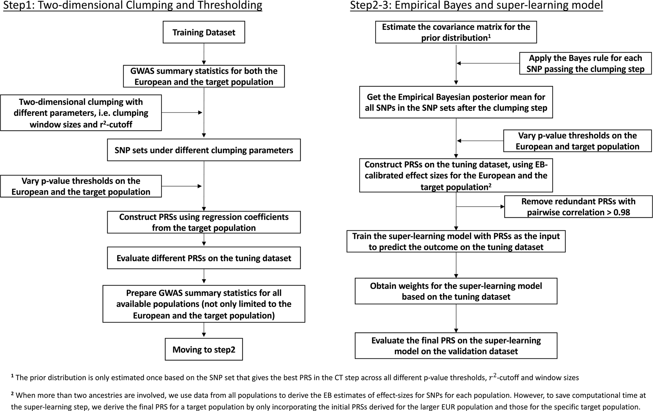
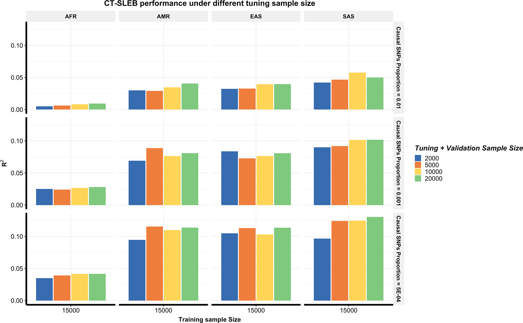
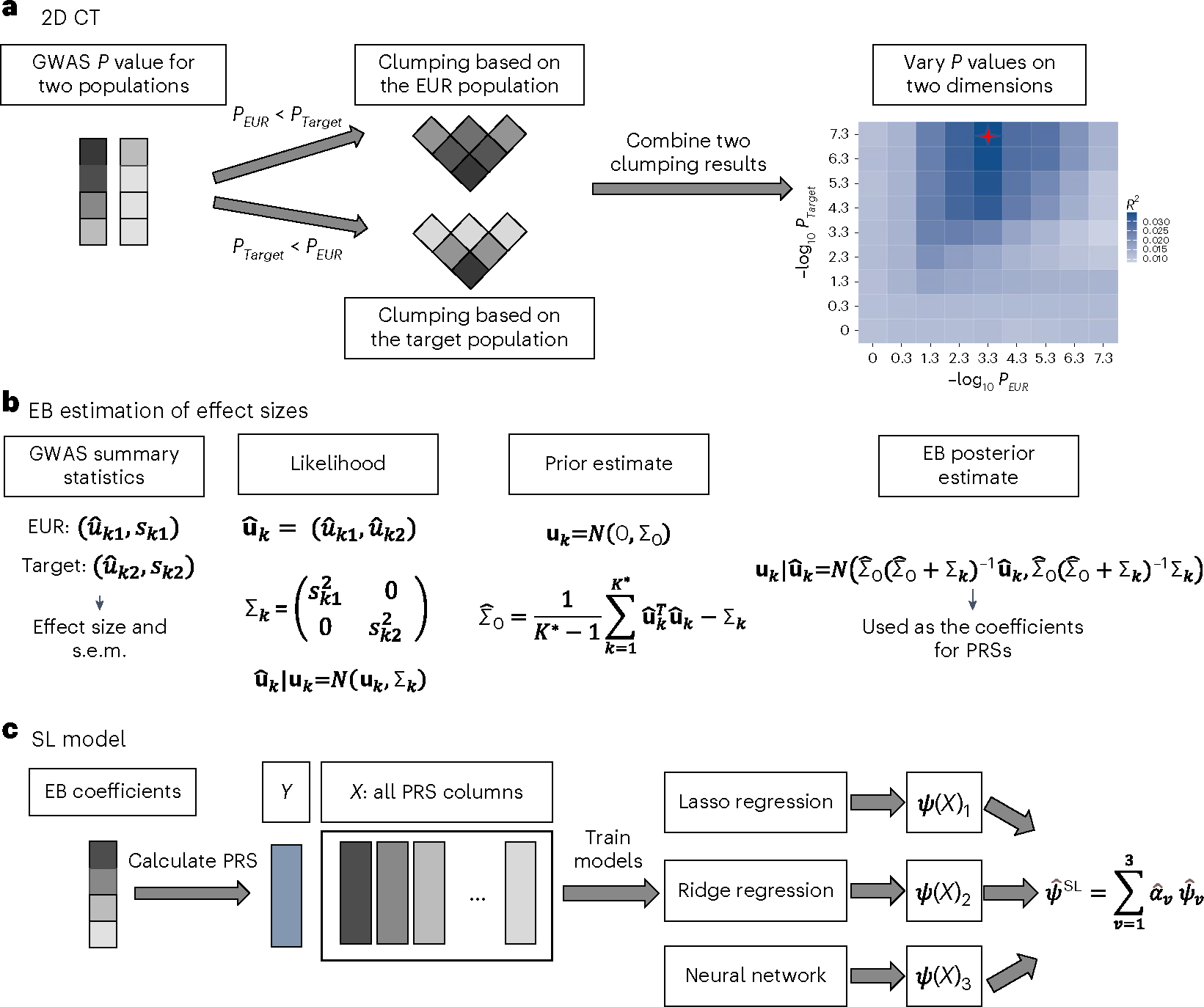
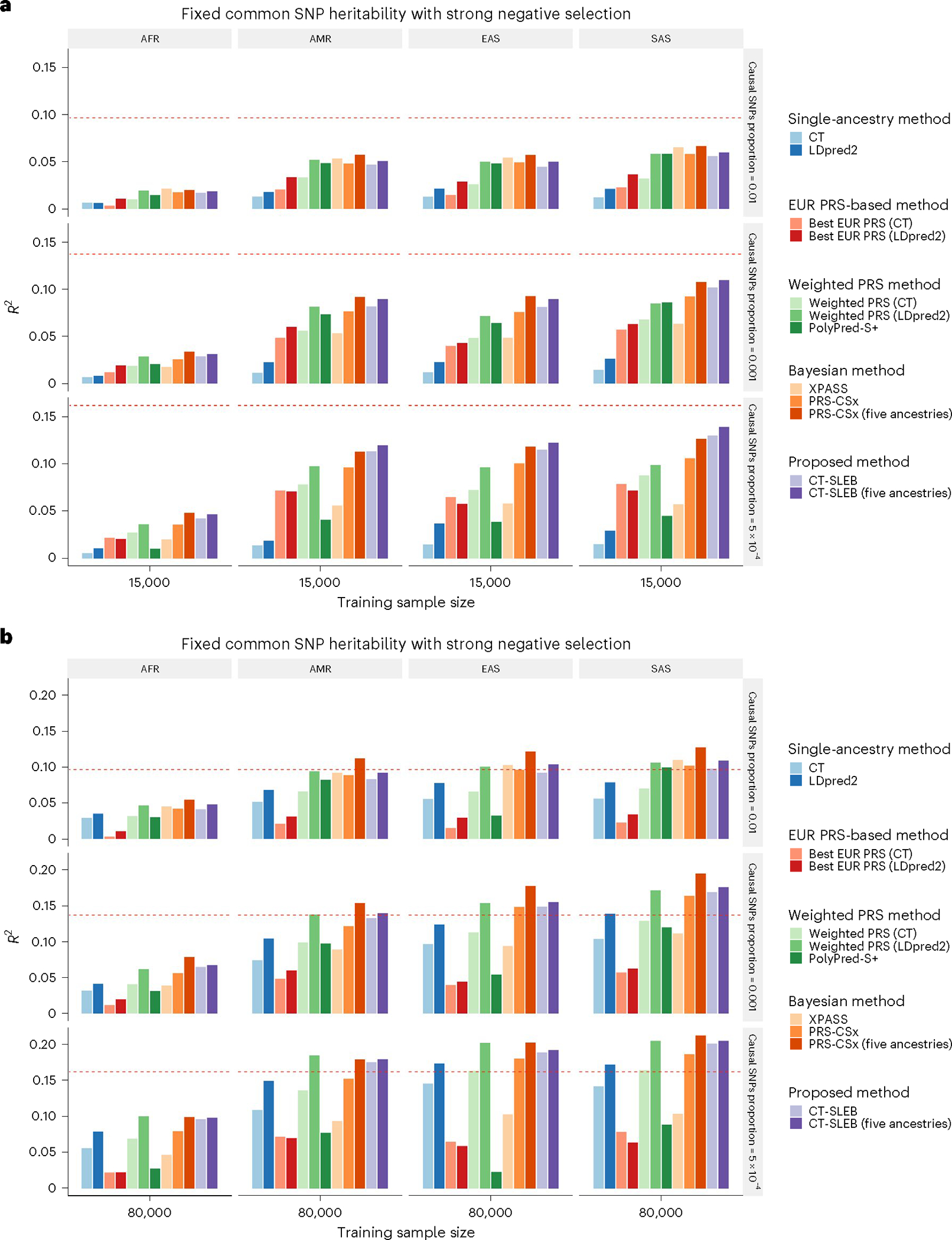
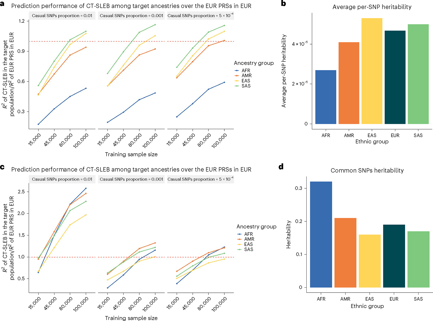
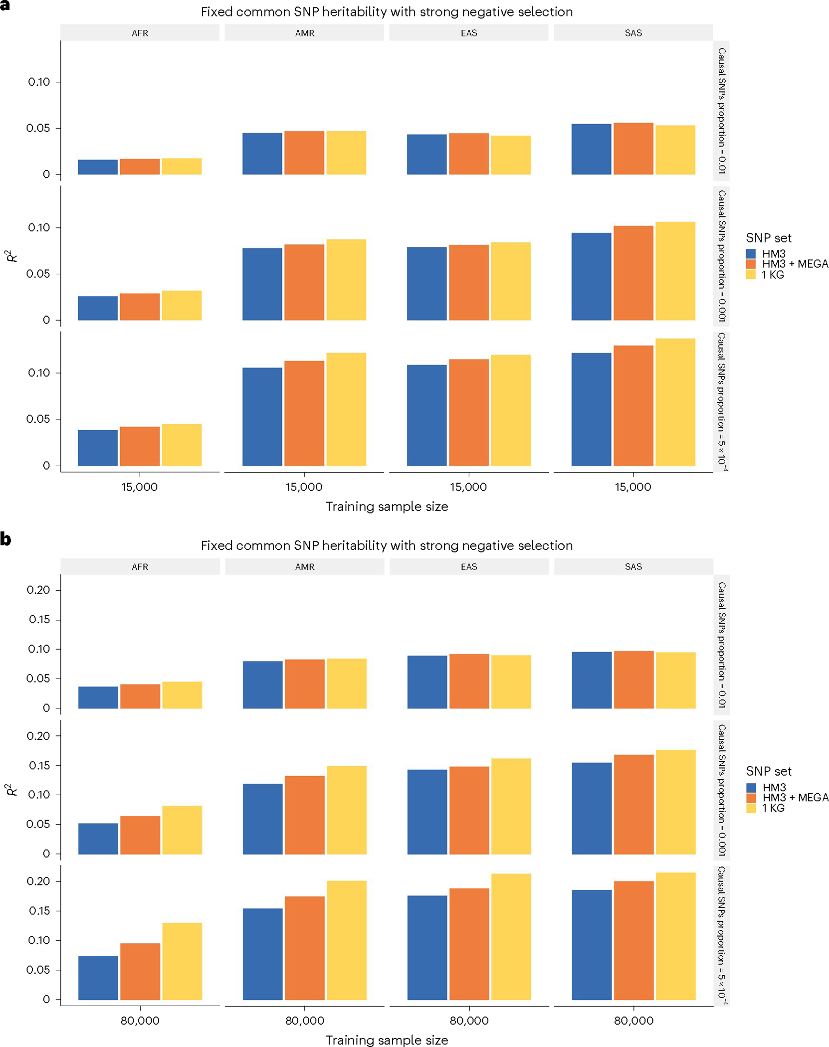
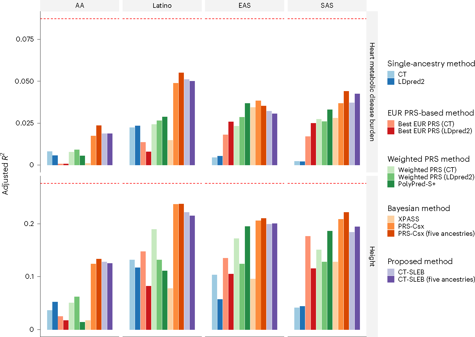
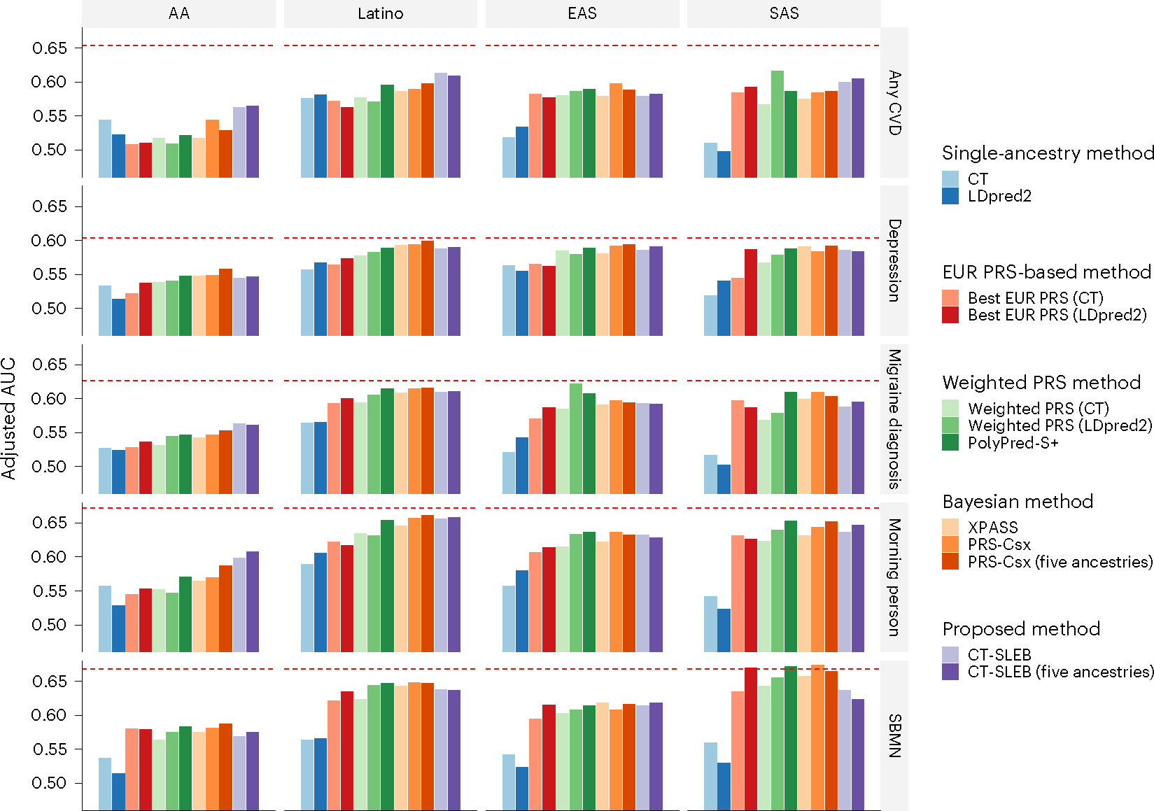
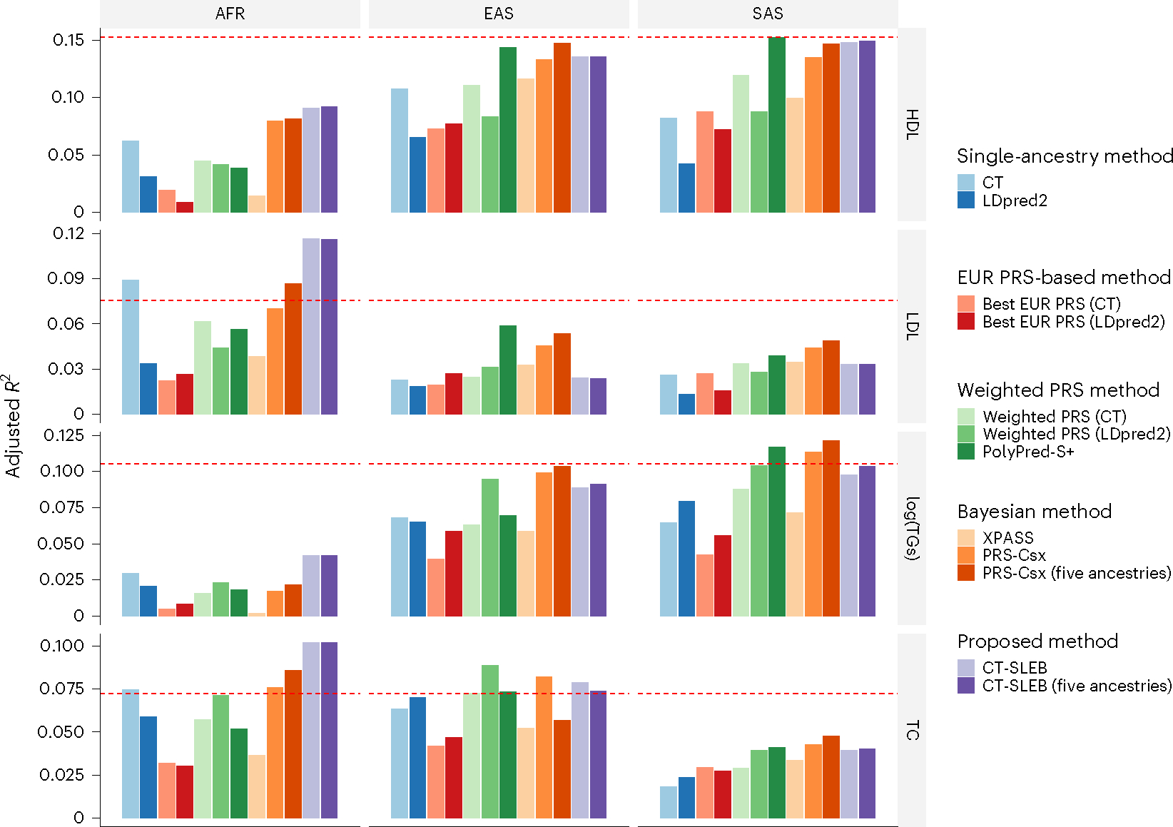
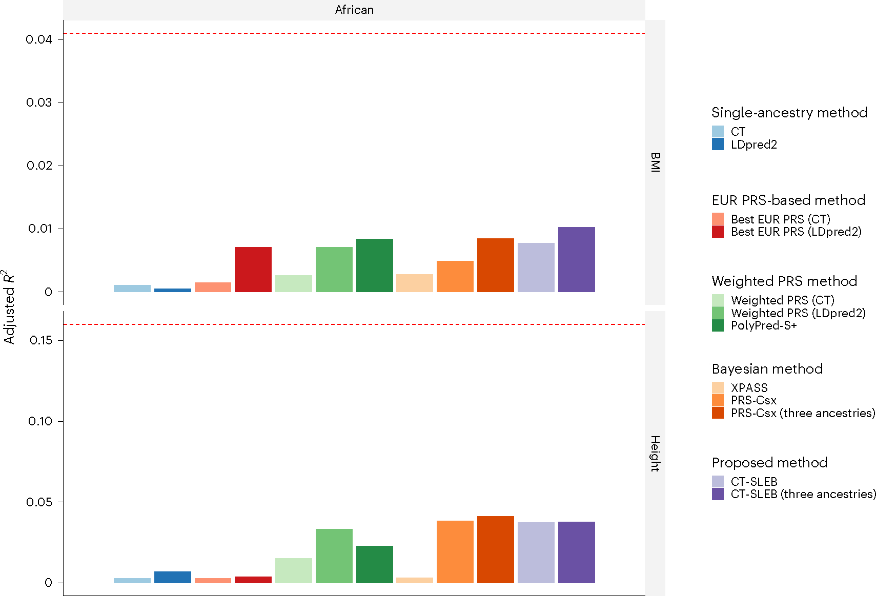
Polygenic risk scores (PRSs) increasingly predict complex traits; however, suboptimal performance in non-European populations raise concerns about clinical applications and health inequities. We developed CT-SLEB, a powerful and scalable method to calculate PRSs, using ancestry-specific genome-wide association study summary statistics from multiancestry training samples, integrating clumping and thresholding, empirical Bayes and superlearning. We evaluated CT-SLEB and nine alternative methods with large-scale simulated genome-wide association studies (~19 million common variants) and datasets from 23andMe, Inc., the Global Lipids Genetics Consortium, All of Us and UK Biobank, involving 5.1 million individuals of diverse ancestry, with 1.18 million individuals from four non-European populations across 13 complex traits. Results demonstrated that CT-SLEB significantly improves PRS performance in non-European populations compared with simple alternatives, with comparable or superior performance to a recent, computationally intensive method. Moreover, our simulation studies offered insights into sample size requirements and SNP density effects on multiancestry risk prediction.

Extended Data Fig. 1 |. CT-SLEB detailed flowchart.

The method contains three major steps: 1. Two-dimensional clumping and thresholding; 2. Empirical-Bayes procedure for utilizing genetic correlations of effect sizes across populations; 3. Super-learning model for combining PRSs under different tuning parameters. The tuning dataset is used to train the super learning model. The final prediction performance is evaluated based on an independent validation dataset. For continuous traits, the prediction is evaluated using R² obtained from the linear regression between outcome and PRS after adjusting for covariates (Methods). For binary traits, the prediction is evaluated using the area under the ROC curve (AUC).

Extended Data Fig. 2 |. Performance of CT-SLEB with different tuning and validation sample sizes.

The total tuning and validation sample size is set as 2000, 5000, 100,000 and 200,000 with half for tuning and half for validation. Analyses are conducted in the multiancestry setting under a strong negative selection model. The training sample size for the AFR population is 15,000. The training sample size for EUR is 100,000. The sample size for the tuning dataset and validation for each population is fixed at 10,000, respectively. Common SNP heritability is assumed to be 0.4 across all populations and effect-size correlation is assumed to be 0.8 across populations. The causal SNPs proportion is varied across 0.01 (top panel), 0.001 (medium panel), or 5 × 10⁻⁴ (bottom panel). The final prediction R² is reported as the average of ten independent simulation replicates.

Fig. 1 |. CT-SLEB workflow.

a–c, The method has three key steps: CT method for selecting SNPs (a); EB procedure for incorporating correlation in effect sizes of genetic variants across populations (b); and SL model for combining the PRSs derived from the first two steps under different tuning parameters (c). GWAS summary statistics data were obtained from the training data. The tuning dataset was used to train the SL model. The final prediction performance was evaluated using an independent validation dataset. s.e.m., standard error of the mean.

Fig. 2 |. Simulation results of various PRS methods in multiancestry settings.

a,b, Each of the four non-EUR populations with a training sample size of 15,000 (a) or 80,000 (b). For the EUR population, the size of the training sample was set at 100,000. The tuning dataset included 10,000 samples per population. Prediction R² values were reported based on an independent validation dataset with 10,000 subjects per population. Common SNP heritability was assumed to be 0.4 across all populations, and effect-size correlation was assumed to be 0.8 across all pairs of populations. The proportion of causal SNPs varies across 0.01 (top), 0.001 (middle), 5 × 10⁻⁴ (bottom), and effect sizes for causal variants are assumed to be related to allele frequency, under a strong negative selection model. Data were generated based on ~19 million common SNPs across the 5 populations, but analyses were restricted to ~2.0 million SNPs that were used on Hapmap3 + MEGA chip array. PolyPred-S+ and PRS-CSx analyses were further restricted to ~1.3 million HM3 SNPs. All approaches were trained using data from the EUR and target populations. CT-SLEB and PRS-CSx were also evaluated using data from all five ancestries as training data. The red dashed line shows the prediction performance of EUR PRSs generated using the single-ancestry method (best of CT or LDpred2) in the EUR population.

Fig. 3 |. Comparison of CT-SLEB PRSs across different ancestries with single-ancestry EUR PRSs in the EUR population.

a–d, The training sample size for each of the four non-EUR populations is 15,000, 45,000, 80,000 or 100,000. The training sample size for the EUR population is fixed at 100,000 and PRS performance is evaluated using single-ancestry CT or LDpred2, depending on whichever performs the best in each setting. a,b, Under the genetic architecture where common SNP heritability is fixed at 0.4, (a) depicts the relative performance of CT-SLEB in non-European populations compared to EUR PRSs, while (b) shows the averaged per-SNP heritability across different ancestries. Then under the genetic architecture where per-SNP heritability is fixed. c,d, (c) demonstrates the relative performance of CT-SLEB in non-European populations relative to EUR PRSs.) The effect-size correlation was assumed to be 0.8 across all pairs of populations. The effect sizes for causal variants were assumed to be related to allele frequency under a strong negative selection model. CT-SLEB uses the summary statistics from all five ancestries.

Fig. 4 |. Prediction performance of CT-SLEB PRS under varying SNP densities.

a,b, The analysis of simulated data based on ~19 million SNPs was limited to 3 different SNP sets: Hapmap3 (~1.3 million SNPs), Hapmap3 + MEGA chips array (~2.0 million SNPs) and 1000 Genomes Project (1KG; ~19 million SNPs). a,b, The training sample size for each of the four non-EUR populations was 15,000 (a) or 80,000 (b). The training sample size for the EUR population was fixed at 100,000. Prediction R² values are reported based on an independent validation dataset with 10,000 subjects per population. Common SNP heritability was assumed to be 0.4 across all populations and effect-size correlation was assumed to be 0.8 across all pairs of populations. The proportion of causal SNPs varied across 0.01 (top), 0.001 (middle) and 5 × 10⁻⁴ (bottom). Lastly, effect sizes for causal variants were assumed to be related to allele frequency under a strong negative selection model.

Fig. 5 |. Prediction accuracy of PRSs for heart metabolic disease burden and height in 23andMe, Inc. datasets.

The total sample size for heart metabolic disease burden and height was, respectively, 2.46 million and 2.93 million for EUR, 131,000 and 141,000 for AFR, 375,000 and 509,000 for Latino, 110,000 and 121,000 for EAS and 29,000 and 32,000 for SAS, respectively. The dataset was randomly split into 70%, 20%, and 10% for training, tuning, and validation datasets, respectively. The adjusted R² values were reported based on the PRS performance in the validation dataset, accounting for PCs 1–5, sex, and age. The red dashed line represents the prediction performance of EUR PRS generated using a single-ancestry method (best of CT or LDpred2) in the EUR population. Analyses were restricted to ~2.0 million SNPs that are included in Hapmap3, or the MEGA chips array or both. PolyPred-S+ and PRS-CSx analyses were further restricted to ~1.3 million HM3 SNPs. All approaches were trained using data from the EUR and the target population. CT-SLEB and PRS-CSx were also evaluated using training data from all five ancestries. From top to bottom, two continuous traits are displayed in the following order: (1) heart metabolic disease burden and (2) height.

Fig. 6 |. Prediction accuracy of five binary traits in 23andMe, Inc. datasets.

The data are from five populations: EUR (averaged n ≈ 2.37 million), AFR (averaged n ≈ 109,000), Latino (averaged n ≈ 401,000), EAS (averaged n ≈ 86,000) and SAS (averaged n ≈ 24,000). The datasets are randomly split into 70%, 20% and 10% for training, tuning and validation datasets, respectively. The adjusted AUC values were reported based on the validation dataset accounting for PCs 1–5, sex and age. The red dashed line represents the prediction performance of EUR PRS generated using a single-ancestry method (best of CT or LDpred2) in the EUR population. Analyses were restricted to the ~2.0 million SNPs that are included in Hapmap3, the MEGA chips array or both. PolyPred-S+ and PRS-CSx analyses were further restricted to ~1.3 million HM3 SNPs as implemented in the provided software. All approaches were trained using data from the EUR and the target populations. CT-SLEB and PRS-CSx were also evaluated using training data from five ancestries. From top to bottom, five binary traits are displayed in the following order: (1) any CVD; (2) depression; (3) migraine diagnosis; (4) SBMN; and (5) morning person.

Fig. 7 |. Prediction accuracy of four blood lipid traits from the GLGC.

We used the GWAS summary statistics from five populations as the training data: EUR (n ≈ 931,000), AFR (primarily AA, n ≈ 93,000), Latino (n ≈ 50,000), EAS (n ≈ 146,000) and SAS (n ≈ 34,000). The tuning and validation datasets are from UKBB data with three different ancestries: AFR (n = 9,042), EAS (n = 2,009) and SAS (n = 10,615). The tuning and validation were split half and half. The adjusted R² values were reported based on the performance of the PRS in the validation dataset, while accounting for PCs 1–10, sex and age. The red dashed line represents the prediction performance of EUR PRSs generated using a single-ancestry method (best of CT or LDpred2) in the EUR population. Analyses were restricted to ~2.0 million SNPs that are included in Hapmap3, the MEGA chips array or both. PolyPred-S+ and PRS-CSx analyses were further restricted to ~1.3 million HM3 SNPs as implemented in the provided software. All approaches were trained using data from the EUR and the target populations. CT-SLEB and PRS-CSx were also evaluated using training data from five ancestries. From top to bottom, four traits are displayed in the following order: (1) HDL-cholesterol, (2) LDL-cholesterol, (3) log(TGs) and (4) TC.

Fig. 8 |. Prediction accuracy of two traits from the AoU dataset.

We used the GWAS summary statistics from three populations as the training data: EUR (n ≈ 48,000), AFR (n ≈ 22,000) and Latino (averaged n ≈ 15,000). The tuning and validation datasets are from UKBB data with AFR (n = 9,042). The tuning and validation were split half and half. The adjusted R² values were reported based on the performance of the PRSs in the validation dataset, while accounting for PCs 1–10, sex and age. The red dashed line represents the prediction performance of EUR PRSs generated using a single-ancestry method (best of CT or LDpred2) in the EUR population. Analyses were restricted to around 800,000 SNPs that were genotyped in the AoU dataset for different ancestries. All approaches were trained using data from the EUR and AFR populations. CT-SLEB and PRS-CSx were further evaluated using training data from three ancestries: AFR, EUR and Latino. From top to bottom, two traits are displayed in the following order: (1) BMI and (2) height.

References

1. Buniello A et al. The NHGRI-EBI GWAS Catalog of published genome-wide association studies, targeted arrays and summary statistics 2019. Nucleic Acids Res. 47, D1005–D1012 (2019). - PMC - PubMed
1. Chatterjee N, Shi J & García-Closas M Developing and evaluating polygenic risk prediction models for stratified disease prevention. Nat. Rev. Genet. 17, 392–406 (2016). - PMC - PubMed
1. Khera AV et al. Genome-wide polygenic scores for common diseases identify individuals with risk equivalent to monogenic mutations. Nat. Genet. 50, 1219–1224 (2018). - PMC - PubMed
1. Mavaddat N et al. Polygenic risk scores for prediction of breast cancer and breast cancer subtypes. Am. J. Hum. Genet. 104, 21–34 (2019). - PMC - PubMed
1. Jia G et al. Evaluating the utility of polygenic risk scores in identifying high-risk individuals for eight common cancers. JNCI Cancer Spectr. 4, pkaa021 (2020). - PMC - PubMed
Publication types