A quantum engine in the BEC-BCS crossover

Abstract

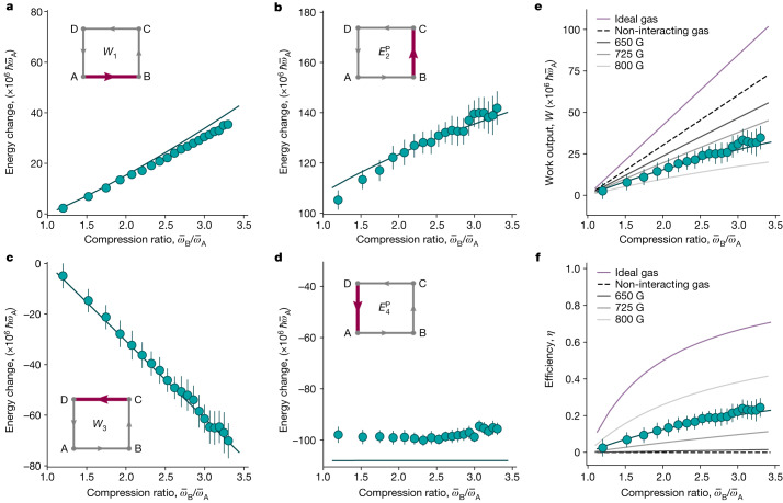
Heat engines convert thermal energy into mechanical work both in the classical and quantum regimes¹. However, quantum theory offers genuine non-classical forms of energy, different from heat, which so far have not been exploited in cyclic engines. Here we experimentally realize a quantum many-body engine fuelled by the energy difference between fermionic and bosonic ensembles of ultracold particles that follows from the Pauli exclusion principle². We employ a harmonically trapped superfluid gas of ⁶Li atoms close to a magnetic Feshbach resonance³ that allows us to effectively change the quantum statistics from Bose-Einstein to Fermi-Dirac, by tuning the gas between a Bose-Einstein condensate of bosonic molecules and a unitary Fermi gas (and back) through a magnetic field^4-10. The quantum nature of such a Pauli engine is revealed by contrasting it with an engine in the classical thermal regime and with a purely interaction-driven device. We obtain a work output of several 10⁶ vibrational quanta per cycle with an efficiency of up to 25%. Our findings establish quantum statistics as a useful thermodynamic resource for work production.

Fig. 1. Principles of the quantum Pauli engine.

a, Schematic of the experimental set-up. The atom cloud (purple ellipsoid) is trapped in the combined fields of a magnetic saddle potential (orange surface) and an optical dipole trap potential (blue cylinder) operating at a wavelength of 1,070 nm. The absorption pictures are taken with an imaging beam (purple arrow) in the −z direction. The scale bar on the absorption picture corresponds to 50 μm. b, Cycle of the Pauli engine. Starting with a molecular BEC that macroscopically populates the ground state of the trap at well-defined temperature T (point A), the first step, A → B, performs work W₁ on the system by compressing the cloud through an increase of the radial trap frequency ${\overline{\omega }}_{\mathrm{B}}>{\overline{\omega }}_{\mathrm{A}}$. This is achieved by enhancing the power of the trapping laser. The second stroke, B → C, increases the magnetic field strength from B_A = 763.6 G (76.36 mT) to the resonant field B_C = 832.2 G, while keeping the trap frequency constant. This leads to a change in the quantum statistics of the system as the working medium now forms a Fermi sea with an associated addition of Pauli energy $E_2^{\mathrm{P}}$, which substitutes the heat stroke. Step C → D expands the trap back to the frequency ${\overline{\omega }}_{\mathrm{A}}$ and corresponds to the second work stroke W₃. Finally, the system is brought back to the initial state with bosonic quantum statistics during step D → A by reducing B_C to B_A, which corresponds to a change in the Pauli energy $E_4^{\mathrm{P}}$. The population distributions in the harmonic trap of the atoms with spin up (blue) and spin down (red) are indicated at each corner. c, Examples of absorption pictures at each point of the engine cycle, where the particular change in size from B → C is due to the Pauli stroke indicating that the Pauli energy increases the size of the cloud in the external potential. Scale bars, 50 μm.

Fig. 2. Contribution of the Pauli energy.

a,b, Trap energy variation ΔU as a function of the number of atoms in a single spin state $N_{\mathrm{A}}^i$ for the magnetic field change between cycle points B → C for a gas performing a Pauli stroke (bringing the gas from a molecular BEC to a unitary gas, cyan), a Feshbach stroke (always remaining in the molecular BEC regime, orange) and a thermal stroke for the same magnetic fields as in the Pauli stroke (red). Symbols represent mean values of 20 repetitions; solid lines are predictions of our model. Owing to the much increased temperature of the gas in the thermal case, trap depth and compression ratio have been chosen differently in the experimental realization to be for the Pauli and Feshbach strokes: T ≈ 120 nK, T/T_F ≈ 0.3 (measured in the molecular BEC regime) and ${\overline{\omega }}_{\mathrm{B}}/{\overline{\omega }}_{\mathrm{A}}=1.5$ (a); and for the thermal stroke: T ≈ 1,150 nK, T/T_F ≈ 0.7 (measured in the molecular BEC regime) and ${\overline{\omega }}_{\mathrm{B}}/{\overline{\omega }}_{\mathrm{A}}=1.1$ (the higher temperature also means that fewer atoms are lost by evaporation) (b). The insets show microscopic sketches of the quantum state of the gas, transitioning between the molecular BEC and Fermi sea, remaining in the molecular BEC, or transitioning between a gas of free molecules to a gas of free atoms, respectively. The error bars for all data points denote 1σ statistical fluctuations of 20 repetitions. c, Pressure–volume (p–V) diagram of the Pauli engine for different compression ratios (black solid and dashed lines). The blue (red) line indicates the equation of state of the Fermi gas (molecular BEC). Varying the compression ratio moves the state of the gas along each line, effectively changing the engine points B and C, whereas the Pauli strokes (bosonization and fermionization) induce transitions between the red and blue lines.

Fig. 3. Performance of the Pauli engine.

a–d, Work contributions, W₁ (a) and W₃ (c), and Pauli energies, $E_2^{\mathrm{P}}$ (b) and $E_4^{\mathrm{P}}$ (d), as a function of the compression ratio ${\overline{\omega }}_{\mathrm{B}}/{\overline{\omega }}_{\mathrm{A}}$ for fixed ${\overline{\omega }}_{\mathrm{A}}$ and fixed number of atoms $N_{\mathrm{A}}^i\approx 2.5\times 10^5$ at point A. The experimental data points (cyan dots) are the mean value of 20 repetitions and the error bars indicate their 1σ statistical uncertainty. The numerical calculations are indicated by the (cyan) solid lines. The insets show the corresponding stroke. e,f, Work output W (e) and efficiency η (f). The experimental points and the numerical simulations are in cyan. For comparison, the W and η values for a non-interacting gas are depicted as black dashed lines. They have been obtained by setting the s-wave scattering length a to zero for points A and B (this limit corresponds to a magnetic field B_A far below the resonance, leading to point-like composite bosons with infinite binding energy) and using the formulas for the energy at unitarity for points C and D. Also, W and η for an ideal gas are shown as purple solid lines and mark the upper bounds of the machine. They have been obtained by using the energy of ideal gases in the degenerate regime (Bose gas for points A and B and Fermi gas for points C and D). The grey solid lines are the theoretical values obtained for different magnetic fields: B_A = 800 G, 725 G and 650 G from lighter to darker (dimer–dimer interaction strength g/g₀ = 2.53, 0.51 and 0.16, respectively, with g₀ being the interaction strength for B_A = 763.3 G).

Fig. 4. Comparison of the performance of quantum many-body devices.

a,b, Work output (a) and efficiency (b) as a function of the number of atoms $N_{\mathrm{A}}^i$ in one spin state for a compression ratio ${\overline{\omega }}_{\mathrm{B}}/{\overline{\omega }}_{\mathrm{A}}=1.5$ for the Pauli engine (cyan dots) and the Feshbach cycle (orange diamonds). Small symbols denote individual realizations; large symbols indicate mean values of 20 repetitions with error bars indicating 1σ statistical fluctuations. For comparison, calculations for a non-interacting gas (black dashed line) and an ideal gas (purple solid line) are shown. Dotted lines are fits to the respective work output W ∝ N^α. The fitted exponents α are 1.73(18) and 1.58(13) for the Pauli engine and Feshbach cycle, respectively, well reproduced by our theoretical model (solid cyan and orange lines). Importantly, the efficiency of the Feshbach cycle is essentially zero. c, Accumulated work output (cyan dots) and efficiency (blue triangles) of the Pauli engine over several cycles for a compression ratio ${\overline{\omega }}_{\mathrm{B}}/{\overline{\omega }}_{\mathrm{A}}=1.5$ and an initial number of atoms in one spin state of about Nⁱ = 2.5 × 10⁵.

Extended Data Fig. 1. Sequence of the Pauli engine cycle.

Magnetic field strength (cyan) and power of the ODT laser (orange). The imaging points during the cycle are marked with purple arrows (A denotes the first point of the cycle and A₂ the last one after a full cycle).

Extended Data Fig. 2. Determination of the correction factor of the number of atoms on resonance for the Pauli engine.

Measured number of atoms of one spin state Nⁱ in point B (red), C (orange), and return to point B_return after reaching point C (purple) in dependence of the number of atoms of one spin state $N_{\mathrm{A}}^i$ in point A. The measured number of atoms in point C cannot differ from the number of atoms in points B and B_return, when the later are equal. Therefore, the measured number of atoms on resonance is higher than the actual number of atoms. Data points are averages of ten repetitions, uncertainties indicate one standard deviation. The inset shows the calculated deviation $N_{\mathrm{C}}/N_{{\mathrm{B}}_{\mathrm{return}}}-1$ (orange points) for the number of atoms on resonance in dependence of $N_{\mathrm{A}}^i$. The mean value of these deviations is 15 % and is visible as a black line, their standard deviation is the grey area. The x-axis of the inset spans the same range as the main axis.

Extended Data Fig. 3. Atom-number correction in the Pauli cycle.

Corrected number of atoms of one spin state Nⁱ in the points of the cycle A (first point of the cycle, black solid line), B (red), C (orange), D (purple), and A₂ (last point of the cycle, cyan) in dependence of the corrected number of atoms of one spin state $N_{\mathrm{A}}^i$ in point A. Experimental data belong to the Pauli engine in Fig. 4(a) and (c) with a compression ratio of ${\overline{\omega }}_{\mathrm{B}}/{\overline{\omega }}_{\mathrm{A}}=1.5$, the number of atoms is experimentally varied. Uncertainty is the standard deviation of 20 repetitions.

Extended Data Fig. 4. Realization of the Pauli engine.

(a)-(d) Measured radii R_mBEC and $R_{\mathrm{res}}$ at each point of the cycle as a function of the compression ratio ${\overline{\omega }}_{\mathrm{B}}/{\overline{\omega }}_{\mathrm{A}}$ for constant number of atoms $N_{\mathrm{A}}^i=2.5\times 10^5$. Radii are extracted by fits of the density profiles with equations (2) or (3). Radii are shown in x-direction (cyan circles) and y-direction (purple triangles). Experimental data are the mean value of 20 repetitions and the corresponding error bars indicate the propagation of the uncertainty of standard deviation of the measurement parameters. The insets show schematics of the cycle, where the point at which the measurement is taken is highlighted (purple). In (d), we compare the experimental values of the radii for A (first point of the cycle) in grey with the last point of the cycle A₂ in the x (y) direction. The trap frequency ${\overline{\omega }}_{\mathrm{B}}$ has no influence on the first measurement point A and ${\overline{\omega }}_{\mathrm{A}}$ is constant for the different compression ratios. Therefore, this setting is only measured once with 20 repetitions. The experimental radii in A₂ (last point of the cycle) are measured after running a full cycle (data points). On the right two exemplary absorption pictures at point C are shown.

Extended Data Fig. 5. Measured temperature T for point A after ramping the magnetic field directly to 680 G (black line).

Uncertainty is the standard deviation of ten repetitions (grey area). The cloud is compressed by increasing the mean trap frequency in stroke A → B. Afterwards, inverting the cycle direction leads again to point A. There, the temperature measurement is repeated after ramping the magnetic field to 680 G (cyan data points). Error bars show the standard deviation of ten repetitions. For comparison, critical temperature (purple solid line) and Fermi temperature (orange solid line) are depicted for point A. Shaded area shows the uncertainty and is of the order of the line thickness.

Extended Data Fig. 6. Realization of the Pauli engine.

Energies (a) E_B, (b) E_C, (c) E_D, and (d) E_A (first point of the cycle) and $E_{{\mathrm{A}}_{\mathrm{2}}}$ (last point of the cycle) at each point of the cycle as a function of the compression ratio ${\overline{\omega }}_{\mathrm{B}}/{\overline{\omega }}_{\mathrm{A}}$ for constant number of atoms Nⁱ ≈ 2.5 × 10⁵. Experimental data (cyan points) are the mean value of 20 repetitions and the corresponding error bars indicate the propagation of uncertainty of standard deviation of the measurement parameters. The experimental data fits well to numerical calculations (cyan solid line), except for point A₂ in (d) because of atom losses. The insets show schematics of the engine with the individually points of the engine highlighted in purple. In (d) the experimental value of the energy E_A is shown in grey for comparison to A₂. The trap frequency ${\overline{\omega }}_{\mathrm{B}}$ has no influence in the first measurement at point A, and ${\overline{\omega }}_{\mathrm{A}}$ is constant for the different compression ratios. Therefore, E_A is only measured once with 20 repetitions.

Extended Data Fig. 7. Pressure and volume for the Pauli engine.

Volume V and pressure p (panel (a) and (b) respectively) for each point of the Pauli cycle: B (red), C (orange), D (purple), and A₂ (last point of the cycle, cyan). The measurements corresponds to the same ones as in Fig. 3 of the main text. The data for the volume are the mean value of 20 repetitions with error bars that lie inside the point size, the error bars in the pressure indicate the propagation of uncertainty of standard deviation of the measurement parameters.

References

1. Callen HB. Thermodynamics and an Introduction to Thermostatistics. Wiley; 1985.
1. Massimi M. Pauli’s Exclusion Principle: The Origin and Validation of a Scientific Principle. Cambridge Univ. Press; 1999.
1. Chin C, Grimm R, Julienne P, Tiesinga E. Feshbach resonances in ultracold gases. Rev. Mod. Phys. 2010;82:1225–1286.
1. Regal CA, Ticknor C, Bohn JL, Jin DS. Creation of ultracold molecules from a Fermi gas of atoms. Nature. 2003;424:47–50. - PubMed
1. Jochim S, et al. Bose–Einstein condensation of molecules. Science. 2003;302:2101–2103. - PubMed