The location and development of Replicon Cluster Domains in early replicating DNA

Abstract

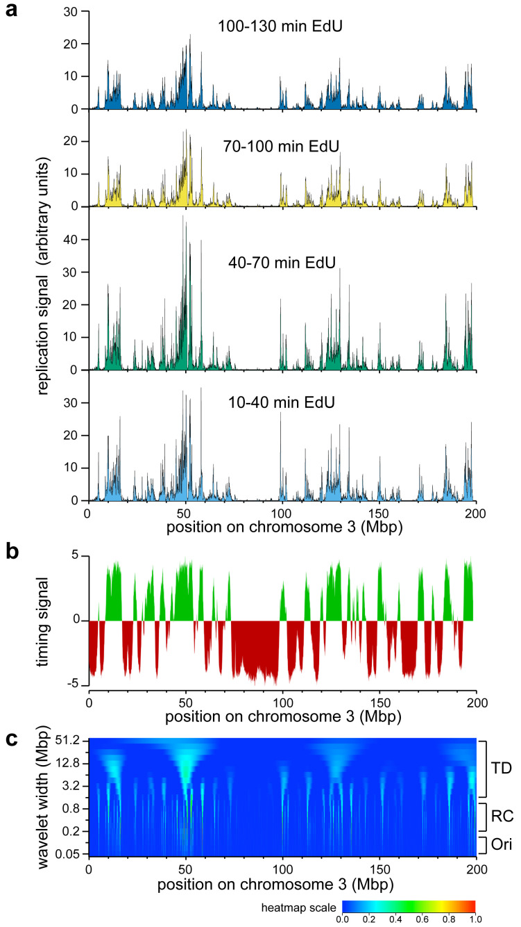
Background: It has been known for many years that in metazoan cells, replication origins are organised into clusters where origins within each cluster fire near-synchronously. Despite clusters being a fundamental organising principle of metazoan DNA replication, the genomic location of origin clusters has not been documented. Methods: We synchronised human U2OS by thymidine block and release followed by L-mimosine block and release to create a population of cells progressing into S phase with a high degree of synchrony. At different times after release into S phase, cells were pulsed with EdU; the EdU-labelled DNA was then pulled down, sequenced and mapped onto the human genome. Results: The early replicating DNA showed features at a range of scales. Wavelet analysis showed that the major feature of the early replicating DNA was at a size of 500 kb, consistent with clusters of replication origins. Over the first two hours of S phase, these Replicon Cluster Domains broadened in width, consistent with their being enlarged by the progression of replication forks at their outer boundaries. The total replication signal associated with each Replicon Cluster Domain varied considerably, and this variation was reproducible and conserved over time. We provide evidence that this variability in replication signal was at least in part caused by Replicon Cluster Domains being activated at different times in different cells in the population. We also provide evidence that adjacent clusters had a statistical preference for being activated in sequence across a group, consistent with the 'domino' model of replication focus activation order observed by microscopy. Conclusions: We show that early replicating DNA is organised into Replicon Cluster Domains that behave as expected of replicon clusters observed by DNA fibre analysis. The coordinated activation of different Replicon Cluster Domains can generate the replication timing programme by which the genome is duplicated.

Keywords: DNA replication; S phase; cell cycle; replication timing; replicon clusters.

Figure 1.. Synchronisation of early S phase cells.

a) Upper panel: description of the procedure for synchronising U2OS cells in early S phase; lower panel: description of method for isolating replicating DNA from synchronised cells. b) Flow cytometry of synchronised cells. Prior to analysis cell cultures were supplemented with EdU for 30 mins at the indicated times after release from L-mimosine. EdU incorporated into DNA was labelled with Alexa Fluor 647 and total DNA was stained with Propidium Iodide. Cells were then analysed by flow cytometry: the x-axis shows DNA content (propidium iodide) and the y-axis EdU content. The red vertical lines indicate the cut-off used in preparative cell sorting experiments to include only cells with a near-G1 DNA content.

Figure 2.. Early replication signals on chromosome 3.

U2OS cells were synchronised in early S phase with thymidine and L-mimosine as described in Figure 1a, and were pulsed for 30 mins with EdU at different times after L-mimosine release. EdU labelled DNA was isolated and sequenced as described in Figure 1a and mapped back to the genome. EdU signals were then normalised to the respective sample’s internal control reference. a) The normalised EdU signals on chromosome 3 are shown for the four time points. b) The replication timing signal for chromosome 3 from https://www2.replicationdomain.com/database.php. Early replicating DNA is shown in green and late replicating DNA in red. c) Heatmap (positive values only) of a wavelet analysis of chromosome 3 using a Ricker wavelet of peak width from 50 kb to 51.2 Mbp, with widths increasing by a factor of √2 between each analysis (log scale) on the y axis. At the bottom of the figure a heatmap colour scheme is shown. Dark blue represents a signal of zero or below and red represents a signal of one. The approximate size of individual replicons (Ori), replicon clusters (RC) and timing domains (TD) are indicated to the right.

Figure 3.. Illustrative results of selected regions on chromosome 3.

Orange bars show the early replication signal from the first time point (EdU labelling from 10–40 mins) on six selected 10 Mbp regions of chromosome 3. Blue lines show the wavelet analysis results with a wavelet peak widths of 500 kb (positive values only). The horizontal dashed line shows the cut-off for calling a wavelet peak as set at the 70 ^th percentile for peaks in late replicating domains (see main text for rationale). Above each replication signal is heatmap of wavelet analysis using a Ricker wavelet of peak widths ranging from 50 kb to 9 Mbp with widths increasing by a factor of √2 between each analysis (log scale) on the y axis and using data in 10 kb bins to allow analysis with the smallest wavelets. The heatmap colour scheme is the same as for Figure 2c.

Figure 4.. Metrics from a genome-wide wavelet analysis.

a, b) The early replication signals from the first time point (EdU labelling from 10–40 mins, brown lines) or an extended first time point (EdU labelling from 0–40 mins, blue lines) with reads mapped onto 50 kb bins (panel a) or 10 kb bins (panel b) were clipped to include only the early timing domains and were analysed using a range of closely-spaced wavelets (peak widths of 100, 150, 200, 250, 300, 350, 400, 450, 500, 550, 600, 650, 700, 750, 800, 1000, 1500 and 3000 kb). Peaks were then called optionally using a minimum peak hight representing the 70 ^th percentile for peaks in late replicating domains (solid lines without cutoff, dashed lines with cutoff). The height of each peak was recorded and the total genome-wide sum for each data point is plotted. c) The early replication signal from the first time point (EdU labelling from 10–40 mins) was clipped to include only the late timing domains and analysed using a wavelet with 500 kb peak width. The peak heights were sorted in order and expressed as a percentile. The early replication signal from the first time point (EdU labelling from 10–40 mins) was then clipped to include only the early timing domains and analysed using a wavelet with 500 kb peak width. Peak calling was then performed using as a cut-off the wavelet peak height at different heights derived from the late-replicating DNA. Solid line shows the number of wavelet peaks (solid line) and the mean wavelet peak height (dashed line) called in the early timing domains using different percentile cut-offs derived from the late timing domains. d) The distribution of wavelet peak heights obtained from applying a wavelet of 500 kb to the first time point (EdU labelling from 10–40 mins) clipped to include only the early timing domains. The darker bar shows the effect of using a 70 ^th percentile cutoff derived from the replication signal in late timing domains, which removes 87 of the smallest wavelet peaks.

Figure 5.. Separation between Replicon Cluster Domains.

A wavelet of width 500 kb was applied to the first time point (EdU labelling from 10–40 mins) clipped to include only the early timing domains (data mapped in 50 kb bins). Wavelet peaks falling below the 70 ^th percentile of peaks identified in late timing domains were removed. The remainder of the peaks were classified as Replicon Cluster Domains. a) The distance between adjacent Replicon Cluster Domains identified within each early timing domain was recorded. The frequency distribution of the separation between adjacent peaks is shown. b) The number of Replicon Cluster Domains identified in each early timing domain is plotted against the size of the early timing domain.

Figure 6.. Exemplar isolated Replicon Cluster Domains.

Six Replicon Cluster Domains that were substantially isolated from other replication signals were chosen as exemplars. Their replication signal in the four time points is shown (light blue, green, yellow and dark blue bars). Each Replicon Cluster Domain was analysed by a series of finely separated wavelets (in 25 kb intervals from 200 kb to 1,200 kb; data in 10 kb bins). The optimal wavelet selected is shown in blue and its width shown in blue text. The same six peaks were fitted to a Gaussian curve which is plotted in red; the red text shows the full width at half maximum of the curve.

Figure 7.. Development of isolated Replicon Cluster Domains.

a) Schematic of an idealised Replicon Cluster Domain containing three active origins. Because of stochasticity in the selection of active origins plus near synchronous initiation within the cluster, as shown in the cartoon to the left, the EdU incorporation profiles on the right would tend to have a flat top and curve down at the edges. The width of the EdU incorporation profiles will expand driven by the outer forks until all internal forks have terminated and incorporation is restricted to the two outer forks. b) Schematic of the EdU incorporation profiles in a single Replicon Cluster Domain in the population of synchronised cells. The green line shows cells where the RCD had become active only in the current timepoint, so its margins more closely match the edges of the RCD. The blue line shows cells where the RCD had become active in a previous timepoint and so its edges will expand due to forks expanding at the margins. The blue-green line shows the observed EdU signal, which comprises elements of both the green and the blue labelling. c- f) The Replicon Cluster Domains from the 10–40 minute EdU data as defined in Figure 5 were filtered to exclude those where the total amount of replication signal in the 500 kb on either side of the wavelet peak was >25% of the replication signal under the wavelet peak. These 123 ‘isolated’ peaks were fitted to an optimal wavelet (using a range of wavelets with peak widths at 25 kb intervals from 200 kb to 1,200 kb; panels c and e) or Gaussian curve (panels d and f) over the four time points. Peaks that fitted to the extreme values of 200 kb or 1,200 kb at any of the four timepoints were rejected. The optimal wavelet width (panel c) or the Gaussian width (panel e) are plotted. The width change between successive time points is plotted in panel d (wavelet) and panel f (Gaussian). The mean width and their standard error for each time point is also listed in panels c and d. The mean width increase between successive times point and its standard error is also listed in panels e and f. g) Statistical analysis of width increases. Mean growth is given in kb/min. CI lo and CI hi are a 95% confidence interval of the mean. The p value is the result of a one sample t-test against zero for peak width increases.

Figure 8.. Examples of valley-filling between Replicon Cluster Domains.

The early replication signal of three selected regions at the four time points is shown as light blue, green, yellow and dark blue bars (data in 50 kb bins). For the first time point (10–40 mins EdU) the wavelet analysis results with a wavelet peak width of 500 kb are shown by the red lines. The horizontal dashed line shows the cut-off for calling a wavelet peak as set at the 70 ^th percentile for peaks in late replicating domains. For the first time point, wavelet peaks are marked by horizontal brown bars; for the successive timepoints the edges of the bars were extended by 90 kb as expected of a fork moving at 1.5 kb/min. At the bottom the relevant timing domain signals for the regions are shown (early timing domains in green and late timing domains in red).

Figure 9.. Analysis of valley-filling genome-wide.

a) Schematic of how ‘valleys’ were analysed genome-wide, using a region on chromosome 8 as an example. The replication signal in the first time point (10–40 mins EdU; 50 kb bins) was subject to wavelet analysis with a wavelet peak width of 500 kb (red lines). For all pairs of wavelet peaks within any given early timing domain, the internal edges of the gap between the edges of the wavelet peaks were reduced by 180 kb to account for fork movement at 1.5 kb/min over two hours; the remaining gap was defined as the ‘valley’. Wavelet analysis with a peak width of 500 kb was then performed on the three later time points, and only those valleys whose flanking wavelet peaks existed (±100 kb error) in all four time points were included for further analysis. For each time point, the mean valley replication signal (horizontal purple line) and minimum valley replication signal (horizontal orange line) were expressed as a percentage of the mean height of the replication signals of the two flanking peaks (black horizontal line). b) The frequency distribution of the mean valley replication signal across the four time points. The mean and standard error of the distribution is also given. c) The frequency distribution of the minimum valley replication signal across the four time points. The mean and standard error of the distribution is also given. d) Statistical analysis of filling rates. Filling rates are given in %/min. CI low and CI high are a 95% confidence interval of the mean. The p value is the result of a one sample t-test against zero.

Figure 10.. Activation order of Replicon Cluster Domains.

The replication signal in the four time points (50 kb bins) was subject to wavelet analysis with a wavelet peak width of 500 kb. Wavelet peaks falling below the 70 ^th percentile of peaks identified in late replicating DNA were removed. The peak height of the replication signal within each wavelet peak was recorded. Groups of peaks were defined by being in the same timing domain and being less than 1600 kb apart. a) Analysis of groups with three members. Each peak was given a rank order dependent on the height of its replication signal and was classified into one of three possible height order permutations (1-2-3, 1-3-2 or 2-1-3). The percentage of groups with each activation sequence over the four time points is shown. Bars showing mean and standard deviation across the four timepoints are also shown. The permutations have been ordered so that moving left to right are permutations that are more ‘domino-like’ and have increasing height similarity. b) Analysis of groups with four members. Each peak was given a rank order dependent on the height of its replication signal and was classified into one of twelve possible height order permutations. The percentage of groups with each activation sequence over the four time points is shown. Bars showing mean and standard deviation across the four timepoints are also shown. The permutations have been ordered so that moving left to right are permutations that are more ‘domino-like’ and have increasing height similarity. c) Schematic showing possible examples of height order groups with 7 peaks. If adjacent peaks have maximal height differences, they will display an interleaved pattern and have a negative score in the adjacent peak similarity metric. If peak heights are randomly distributed they will on average have a zero score in the adjacent peak similarity metric. If peak heights are in perfect (‘domino’) order they will have a score of one in the adjacent peak similarity metric. d) Groups of peaks with four or more members were analysed by the adjacent peak similarity metric, and the frequency distribution in the four different time points is shown. Groups with three members were omitted from this analysis because with only three members the metric cannot distinguish between random and anti-ordered. e) Statistical analysis of the adjacent peak similarity metric. CI low and CI high are a 95% confidence interval of the mean. The p value is the result of a one sample t-test against zero. The ‘no-rep’ p value is a similar one sample t-test against zero where each group of peaks was logged only once (see Methods for details).

References

1. Jain M, Koren S, Miga KH, et al. : Nanopore sequencing and assembly of a human genome with ultra-long reads. Nat Biotechnol. 2018;36(4):338–345. 10.1038/nbt.4060 - DOI - PMC - PubMed
1. Bellush JM, Whitehouse I: DNA replication through a chromatin environment. Philos Trans R Soc Lond B Biol Sci. 2017;372(1731): 20160287. 10.1098/rstb.2016.0287 - DOI - PMC - PubMed
1. Maya-Mendoza A, Tang CW, Pombo A, et al. : Mechanisms regulating S phase progression in mammalian cells. Front Biosci (Landmark Ed). 2009;14(11):4199–4213. 10.2741/3523 - DOI - PubMed
1. Chagin VO, Casas-Delucchi CS, Reinhart M, et al. : 4D Visualization of replication foci in mammalian cells corresponding to individual replicons. Nat Commun. 2016;7: 11231. 10.1038/ncomms11231 - DOI - PMC - PubMed
1. Blow JJ, Ge XQ, Jackson DA: How dormant origins promote complete genome replication. Trends Biochem Sci. 2011;36(8):405–414. 10.1016/j.tibs.2011.05.002 - DOI - PMC - PubMed
LinkOut - more resources