Automated customization of large-scale spiking network models to neuronal population activity

Abstract

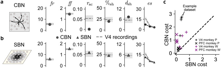
Understanding brain function is facilitated by constructing computational models that accurately reproduce aspects of brain activity. Networks of spiking neurons capture the underlying biophysics of neuronal circuits, yet the dependence of their activity on model parameters is notoriously complex. As a result, heuristic methods have been used to configure spiking network models, which can lead to an inability to discover activity regimes complex enough to match large-scale neuronal recordings. Here we propose an automatic procedure, Spiking Network Optimization using Population Statistics (SNOPS), to customize spiking network models that reproduce the population-wide covariability of large-scale neuronal recordings. We first confirmed that SNOPS accurately recovers simulated neural activity statistics. Then, we applied SNOPS to recordings in macaque visual and prefrontal cortices and discovered previously unknown limitations of spiking network models. Taken together, SNOPS can guide the development of network models and thereby enable deeper insight into how networks of neurons give rise to brain function.

Figure 1:. Framework for automated customization of a spiking network model to neuronal recordings.

a, A SNN has a complicated dependency between its parameters and spiking output. For example, different parameter sets correspond to each of four previously-identified activity regimes of a classical balanced network: asynchronous irregular, synchronous regular, synchronous irregular, and asynchronous regular. In this case, the SNN has a 9-dimensional parameter space. b, Our customization framework matches activity statistics of spike trains produced by the network model to those of neuronal recordings. It uses a guided searching algorithm to iteratively update the model parameters. The activity statistics are defined by the user and can include single-neuron, pairwise, and population activity statistics.

Figure 2:. Activity statistics for comparing the activity of a spiking network model to neuronal recordings.

a, Three types of activity statistics based on single neurons (e.g., firing rate and Fano factor), pairs of neurons (e.g., spike count correlation), and a population of neurons (e.g., percent shared variance, number of dimensions, and eigenspectrum of shared variance). The units of firing rate are spikes per second, those of Fano factor are spike count, and those of the eigenspectrum of shared variance are (spike count). All other activity statistics are unitless. These activity statistics are all based on spike counts within a 200 ms spike count bin (left panel), which can be represented in a population activity space (center panel). Each dot represents the activity across the neuronal population within a given time window. b, Activity statistics based on population recordings in macaque visual area V4 (dashed lines) are challenging to reproduce by the four parameter regimes of a CBN (colored symbols, cf. Fig. 1a, mean across 5 network instantiations of network connectivity graphs and initial membrane potentials corresponding to the same network parameter set). None of the four activity regimes accurately reproduces the activity statistics of the V4 population recordings (dashed lines). The V4 activity statistics are shown as the mean ± 1 SD across 19 recording sessions (see Methods). All activity statistics are based on randomly subsampling 50 neurons from each CBN or V4 dataset.

Figure 3:. Customizing a spiking network model using Bayesian optimization with Gaussian processes.

The Bayesian optimization algorithm attempts to find a parameter set $\theta$ for a spiking network model such that its activity statistics match those of neuronal recordings. a, Spike trains are recorded from the brain and their activity statistics, ${\mathit{s}}_{\text{true}}$, are computed. This step is performed only once, since the same recorded activity is used for comparison on all iterations. b, On the k-th iteration, spike trains are generated from the network model using parameter set ${\theta }_k$, proposed by the previous iteration. c, The activity statistics of the spike trains generated from the network model, $\mathit{s}({\theta }_k)$, are computed. The cost for ${\theta }_k$ depends on how far each of those activity statistics is from the corresponding activity statistics of the neuronal recordings, ${\mathit{s}}_{\text{true}}$. d, A Gaussian process (GP) (solid line) is used to approximate the true, unknown cost function, $c(\theta )$ (red dashed line). We seek to find the minimum of this true, unknown cost function (denoted by ${\theta }^{\star }$). Each iteration of the Bayesian optimization provides one evaluation of the cost at a particular setting of the model parameters (black dots). The cost at the current iteration is labeled $\widehat{c}({\theta }_k)$, and the other black dots represent the costs evaluated during previous iterations. The GP provides an uncertainty of our estimate of the cost function (gray shading). For illustrative purposes, we show here a single model parameter being optimized, whereas our algorithm typically optimizes multiple model parameters simultaneously. e, An acquisition function is defined based on the GP in d to determine the next parameter set, ${\theta }_{k+1}$, to evaluate. The acquisition function implements an exploration-exploitation trade-off, where areas of low predicted cost and high uncertainty are desirable.

Figure 4:. SNOPS accurately customizes a classical balanced network model to simulated spike trains.

a, A CBN was used to generate spike trains with randomly chosen parameter sets ${\theta }_{\text{true}}$ (see Methods). SNOPS (or other optimization algorithms) was then used to customize the parameters, ${\theta }_k$, of a separate CBN to match the “ground truth” activity statistics, ${\mathit{s}}_{\text{true}}$, of the generated spike trains. b, For a given amount of computer running time (see Methods), SNOPS (blue) finds parameters with lower cost than accelerated random search (red) and random search (green). Vertical axis represents the lowest log(cost) up to the given running time and hence decreases monotonically. Solid lines and shading represent the mean ± 1 SD across 40 customization runs. c, For a representative customization run, SNOPS (blue) identified model parameters whose activity statistics were closer to the ground truth (dashed lines) than accelerated random search (red) and random search (green). Error bars on the ground truth represent one SD across 5 network instantiations corresponding to the same ground truth parameter set. Circles represent the mean across 5 network instantiations corresponding to the network parameter set identified by each optimization algorithm. d, Across all 40 customization runs, SNOPS accurately reproduced the ground truth activity statistics (all points lie near the diagonal). Each dot represents the results from one SNOPS customization run to a randomly generated ground truth dataset. For visual clarity, only the first (i.e., most dominant) mode of es is plotted in the rightmost panel.

Figure 5:. The spatial balanced network (SBN) more accurately reproduces activity statistics of macaque V4 and PFC datasets than the classical balanced network (CBN).

a, Left: Stylized representation of the CBN. Right: Activity statistics of the CBN (circles, mean across 5 network instantiations corresponding to the same identified parameter set) after being customized using SNOPS to the same V4 dataset as in Fig. 2b. Dashed line and shading represent the mean ± 1 SD across 19 sessions. b, Left: Stylized representation of the SBN. The SBN is different from the CBN in that the connection probability depends on the distance between neurons. Right: Activity statistics of the SBN (triangles, mean across 5 network instantiations corresponding to the same identified parameter set) after being customized using SNOPS to the same V4 datasets as in a. c, The SBN more accurately reproduced activity statistics than the CBN across 16 datasets, comprising four task conditions with recordings in two brain areas (V4 and PFC) in each of the two monkeys. Arrow indicates the example V4 dataset shown in a and b.

Figure 6:. Trade-off cost reveals the inflexibility of CBN relative to SBN.

a, Activity statistics of the CBN (circles, mean across 5 network instantiations corresponding to the same identified parameter set) and SBN (triangles, mean across 5 network instantiations corresponding to the same identified parameter set) after being customized using SNOPS to one V4 activity statistic (dashed line) at a time. Same V4 dataset as Fig. 2b. b, A high trade-off cost represents the case where customizing the network to reproduce two activity statistics simultaneously yields a higher average cost of the two statistics than customizing each statistic individually (upper panel). By contrast, a low trade-off cost represents the case where the cost of customizing two activity statistics simultaneously yields a similar cost to customizing each statistic individually (lower panel). c, Trade-off costs between pairs of statistics for the CBN (upper panel) and SBN (lower panel) on the same V4 dataset as Fig. 2b. d, Customizing the CBN and SBN to different numbers of activity statistics included in the cost function simultaneously, on the same V4 dataset as Fig. 2b. Each dot represents one particular subset of activity statistics (e.g., highlighted dot indicates the average cost of $r_{\text{sc}}$ and $ff$ when including only those two activity statistics in the cost function). The cost of each dot was computed over 5 network instantiations corresponding to the same identified parameter set of that dot. Each bar indicates the average cost across all subsets of the corresponding number of activity statistics.

References

1. Hodgkin Allan L and Huxley Andrew F. Currents carried by sodium and potassium ions through the membrane of the giant axon of loligo. The Journal of physiology, 116(4):449, 1952. - PMC - PubMed
1. Marder Eve and Bucher Dirk. Understanding circuit dynamics using the stomatogastric nervous system of lobsters and crabs. Annu. Rev. Physiol., 69:291–316, 2007. - PubMed
1. Vogels Tim P, Rajan Kanaka, and Abbott Larry F. Neural network dynamics. Annu. Rev. Neurosci., 28:357–376, 2005. - PubMed
1. Kass Robert E, Amari Shun-Ichi, Arai Kensuke, Brown Emery N, Diekman Casey O, Diesmann Markus, Doiron Brent, Eden Uri T, Fairhall Adrienne L, Fiddyment Grant M, et al. Computational neuroscience: Mathematical and statistical perspectives. Annual review of statistics and its application, 5:183–214, 2018. - PMC - PubMed
1. Wang Xiao-Jing. Theory of the multiregional neocortex: large-scale neural dynamics and distributed cognition. Annual review of neuroscience, 45:533–560, 2022. - PMC - PubMed
Publication types