Neuronal Population Activity in Macaque Visual Cortices Dynamically Changes through Repeated Fixations in Active Free Viewing

Abstract

During free viewing, we move our eyes and fixate on objects to recognize the visual scene of our surroundings. To investigate the neural representation of objects in this process, we studied individual and population neuronal activity in three different visual regions of the brains of macaque monkeys (Macaca fuscata): the primary and secondary visual cortices (V1, V2) and the inferotemporal cortex (IT). We designed a task where the animal freely selected objects in a stimulus image to fixate on while we examined the relationship between spiking activity, the order of fixations, and the fixated objects. We found that activity changed across repeated fixations on the same object in all three recorded areas, with observed reductions in firing rates. Furthermore, the responses of individual neurons became sparser and more selective with individual objects. The population activity for individual objects also became distinct. These results suggest that visual neurons respond dynamically to repeated input stimuli through a smaller number of spikes, thereby allowing for discrimination between individual objects with smaller energy.

Keywords: object recognition.

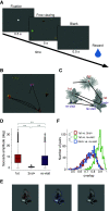
Figure 1.

A, Free viewing task paradigm. The trial starts with the appearance of a fixation spot. The animal needs to fixate on the spot for 0.5 s (here, the fixation spot size is exaggerated). After completion of fixation, an image for free viewing appears. The animal is required to keep its eyes within the monitor screen for 5 s. The liquid reward is delivered after completion of the 5-s free viewing. B, Example visual stimulus image and corresponding eye movement pattern (black lines) and fixation positions (red dots) during one stimulus image presentation. C, Categorization of fixations. D, Saccade amplitude just before the first, second+, and re-visit fixations (n = 91,474, 65,730, and 45,289 for the first, second+, and re-visit, respectively). Horizontal lines are the medians, the upper and lower borders of the boxes are the 25th-75th percentiles, and the upper and lower whiskers represent the maximum and minimum values of nonoutliers. Crosses are outliers. Asterisks indicate statistical significance for the Mann–Whitney U test (p-value = 0 for first vs. second+, 0 for first vs. re-visit, and 0 for second+ vs. re-visit). Extended Data Table 1-1 summarizes the related statistical values. E, Example fixation positions of an object in first (red), second+ (blue), and re-visit (purple) fixations. F, Distribution of fixation position overlaps of the same object between different fixation categories (n = 1176). Asterisks indicate statistical significance for the sign-rank test (p-value = 5.8 × 10⁻¹⁸² for first-second+ vs. first-re-visit and 6.0 × 10⁻¹⁸⁴ for first-re-visit vs. second+-re-visit). Extended Data Table 1-2 summarizes the related statistical values.

Figure 2.

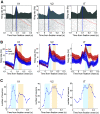
A, Fixation-triggered perifixation time histogram (PFTH) and raster plot of example neurons from each area. The vertical blue line is the peak of the PFTH. Red dots in the raster plot are fixation offsets, i.e., the onset of the next saccade. B, Comparison of the firing rates of different fixation categories. The population mean firing rates of recorded neurons in each area. Colored lines (red, purple, and blue) indicate different fixation categories, with the colored shaded areas indicating the SEM (n = 87, 92, and 337 for V1, V2, and IT, respectively). Asterisks indicate the time points that showed significant differences in the mean firing rates between first and second+ (blue) or first and re-visit (purple) fixations (bin size 1 ms; signed-rank test, p < 0.01, Bonferroni corrected). For comparison, the response to the preferred object is summarized in Extended Data Figure 2-1. C, Number of neurons that showed significant (p < 0.01, rank-sum test, one-sided) decreases in firing rates between the first and later (second+ and re-visit) fixations across time. The light blue and yellow shaded areas in B and C indicate the fixation order-dependent response (FODR) periods 1 and 2, respectively.

Figure 3.

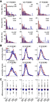
A, Object selectivity of example neurons. Each bar is the mean firing rate for fixation on each object during FODR1. The object IDs are arranged in descending order on the x-axis according to the mean firing rate for first fixations. The error bars are the SEM. B, The number of objects that evoked increased or decreased responses from first to second+ (left) or from first to re-visit (right) fixations calculated during FODR1 or FODR2 (n = 87, 97, and 337 for V1, V2, and IT, respectively). C, Decrease in sparseness in second+ and re-visit fixations compared with first fixations during FODR1 and FODR2. The sparseness of first fixations was subtracted for each neuron. Colors correspond to the fixation orders (n = 85, 95, and 318 for V1, V2, and IT, respectively). The convention for the box plots is the same as in Figure 1D. Asterisks indicate statistical significance for the signed-rank test between first fixations and second+ or re-visit fixations (**p < 0.01). The p-values are 2.4 × 10⁻⁵, 1.5 × 10⁻⁶, 1.5 × 10⁻⁴, and 1.4 × 10⁻⁸ for FODR1-second+, FODR2-second+, FODR1-re-visit, and FODR2-re-visit, respectively, for V1; 2.1 × 10⁻¹⁰, 2.5 × 10⁻¹³, 6.8 × 10⁻¹³, and 4.1 × 10⁻¹⁴ for FODR1-second+, FODR2-second+, FODR1-re-visit, and FODR2-re-visit, for V2; and 5.5 × 10⁻¹⁰, 1.1 × 10⁻¹³, 5.8 × 10⁻²⁴, and 2.3 × 10⁻³¹ for IT). Extended Data Tables 3-1 and 3-2 summarize the related statistical values. The comparison of sparseness across recording areas or across subjects is shown in Extended Data Figure 3-1.

Figure 4.

A, Population activity profiles of example objects. Red and blue correspond to different objects. Each bar corresponds to the mean firing rate of neurons for an object. The neuronal IDs are arranged in descending order on the x-axis according to the mean firing rates for the object shown in the red bar in each fixation category. The cosine similarity of each combination of firing profiles is shown at the top right. B, Cosine similarity distribution calculated for all available object combinations for each fixation category (corresponds to the color; n = 991, 1210, and 2342 for V1, V2, and IT, respectively). Crosses at the top are the means of each distribution. C, Decrease in cosine similarity. Cosine similarities for first fixations were subtracted from those of second+ and re-visit fixations. Colors correspond to the fixation orders (n = 991, 1210, and 2342 for V1, V2, and IT, respectively). The white lines are the medians and the upper and lower borders of the boxes are the 25th–75th percentiles, and the upper and lower whiskers represent the maximum and minimum values of nonoutliers. Crosses are outliers. Asterisks indicate significant differences for the Kolmogorov–Smirnov test (**p < 0.01). The p-values are 1.3 × 10⁻¹⁴ (vs. second+ FODR1), 6.4 × 10⁻¹⁶ (vs. second+ FODR2), 2.2 × 10⁻⁶ (vs. re-visit FODR1), and 2.9 × 10⁻⁵ (vs. re-visit FODR2) for V1; 3.6 × 10⁻¹² (vs. second+ FODR1), 1.0 × 10⁻⁵⁴ (vs. second+ FODR2), 0.8 × 10⁻⁹ (vs. re-visit FODR1), and 6.3 × 10⁻¹⁵ (vs. re-visit FODR2) for V2; and 6.3 × 10⁻⁵¹ (vs. second+ FODR1), 2.3 × 10⁻⁷⁸ (vs. second+ FODR2), 1.2 × 10⁻³⁴ (vs. re-visit FODR1), and 1.1 × 10⁻⁵³ (vs. re-visit FODR2) for IT. Extended Data Tables 4-1 and 4-2 summarize the related statistical values. The comparison of cosine similarity across recording areas or subjects and the effect of reduction of firing rate on cosine similarity is shown in Extended Data Figure 4-1.

Figure 5.

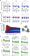
A, Comparison of mean cosine similarities between second1 and second2 fixations for the three areas. The box plot shows the cosine similarities for second1 and second2 subtracted from those of the first fixations. Colors correspond to fixation orders. The convention for the box plots is the same as in Figure 1D. Asterisks indicate significant differences for the Kolmogorov–Smirnov test (**p < 0.01). The p-values are 1.5 × 10⁻¹⁶ (second1 vs. second2 in FODR1 of V1), 1.2 × 10⁻²¹ (FODR2 of V1), 6.9 × 10⁻¹⁰ (FODR1 of V2), 1.2 × 10⁻³⁹ (FODR2 of V2), 2.5 × 10⁻⁴⁷ (FODR1 of IT), and 1.0 × 10⁻⁵⁵ (FODR2 of IT). The black lines are the means (n = 788, 910, and 1832 for V1, V2, and IT, respectively). Extended Data Table 5-1 summarizes the related statistical values. B, Comparison of cosine similarities between re-visit1 and re-visit2 fixations. Conventions are same as in A (n = 534, 620, and 1654 for V1, V2, and IT, respectively). The p-values are 0.11 (re-visit1 vs. re-visit2 in FODR1 of V1), 0.19 (FODR2 of V1), 0.78 (FODR1 of V2), 1.0 (FODR2 of V2), 0.006 (FODR1 of IT, higher for re-visit2), and 0.01 (FODR2 of IT, higher for re-visit2). Extended Data Table 5-2 summarizes the related statistical values. C, Fixation order distribution within 5.0 s of the onset of the free viewing trial. D, Categorization of fixations by mixed-sample ordering. E, Comparison of cosine similarities among fixation orders in mixed-sample ordering (green). For reference, the cosine similarity for a first fixation is shown in red. The red line is the linear fit to the mean cosine similarity across fixation orders (n = 846, 989, and 1835 for V1, V2, and IT, respectively). Extended Data Tables 5-3, 5-4, and 5-5 summarize the related statistical values. For comparison, Extended Data Figure 5-1 summarizes the cosine similarity for the fixation task.

Figure 6.

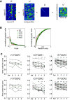
A, Singular value decomposition of an example session of IT (data of FODR1, mix2 fixations). B, Normalized singular values (left) and their cumulative values (right) from the same example session as A. Color corresponds to the saccade orders. C, Area under the curve of all the sessions of different fixation categories (first, and mixed 2, 3, 4, and 5). The red and green crosses are the mean AUC across sessions. Asterisks indicate significant differences for the signed-rank test (*p < 0.05; **p < 0.01). The p-values are 0.063 (vs. mix2), 0.63 (vs. mix3), 0.063 (vs. mix4), and 0.063 (vs. mix5), for V1 of FODR1; 0.063 (vs. mix2), 0.063 (vs. mix3), 0.063 (vs. mix4), and 0.063 (vs. mix5), for V1 of FODR2; 0.014 (vs. mix2), 0.020 (vs. mix3), 2.0 × 10⁻³ (vs. mix4), and 3.9 × 10⁻³ (vs. mix5) for V2 of FODR1; 0.084 (vs. mix2), 2.0 × 10⁻³ (vs. mix3), 2.0 × 10⁻³ (vs. mix4), and 0.039 (vs. mix5) for V2 of FODR2; 2.1 × 10⁻³ (vs. mix2), 1.6 × 10⁻³ (vs. mix3), 4.6 × 10⁻⁴ (vs. mix4), and 1.8 × 10⁻³ (vs. mix5) for IT of FODR1; and 5.4 × 10⁻⁴ (vs. mix2), 1.0 × 10⁻³ (vs. mix3), 2.3 × 10⁻⁴ (vs. mix4), and 3.3 × 10⁻⁴ (vs. mix5) for IT of FODR2. Extended Data Tables 6-1 and 6-2 summarize the related statistical values.

Figure 7.

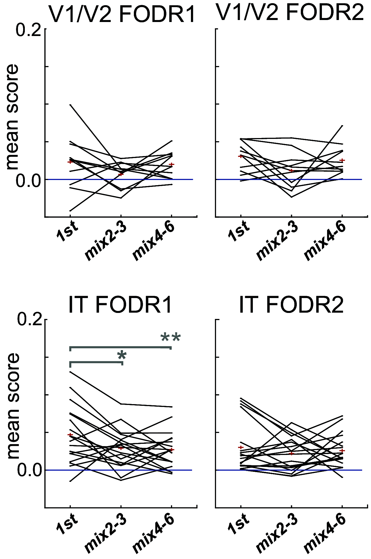
Discrimination accuracy by linear discriminant analysis (LDA) for each area in FODR1 and FODR2. Each line is the 10-fold cross-validation mean score across 10 random selection trials. The chance score calculated by randomization for each session was subtracted [n = 11 (V1/V2), 18 (IT)]. The asterisks indicate significant differences compared with first for the two-sided signed-rank test (*p < 0.05, **p < 0.01). The p-values are 0.17 (vs. mix2–3) and 0.64 (vs. mix4–6) for V1/V2 of FODR1; 0.083 (vs. mix2–3) and 0.46 (vs. mix4–6), for V1/V2 of FODR2; 0.035 (vs. mix2–3), 0.0065 (vs. mix4–6) for IT of FODR1; and 0.27 (vs. mix2–3), and 0.98 (vs. mix4–6) for IT of FODR2. Extended Data Tables 7-1 and 7-2 summarize the related statistical values.

References

1. Auksztulewicz R, Friston K (2016) Repetition suppression and its contextual determinants in predictive coding. Cortex 80:125–140. 10.1016/j.cortex.2015.11.024 - DOI - PMC - PubMed
1. Barlow HB (1972) Single units and sensation: a neuron doctrine for perceptual psychology? Perception 1:371–394. 10.1068/p010371 - DOI - PubMed
1. Brunet NM, Bosman CA, Vinck M, Roberts M, Oostenveld R, Desimone R, Weerd PD, Fries P (2014) Stimulus repetition modulates gamma-band synchronization in primate visual cortex. Proc Natl Acad Sci U S A 111:3626–3631. 10.1073/pnas.1309714111 - DOI - PMC - PubMed
1. Cortes JM, Marinazzo D, Series P, Oram MW, Sejnowski TJ, van Rossum MCW (2012) The effect of neural adaptation on population coding accuracy. J Comput Neurosci 32:387–402. 10.1007/s10827-011-0358-4 - DOI - PMC - PubMed
1. De Baene W, Vogels R (2010) Effects of adaptation on the stimulus selectivity of macaque inferior temporal spiking activity and local field potentials. Cereb Cortex 20:2145–2165. 10.1093/cercor/bhp277 - DOI - PubMed
Publication types
LinkOut - more resources