Surfactant amplifies yield-stress effects in the capillary instability of a film coating a tube

Abstract

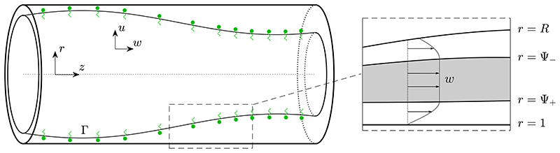
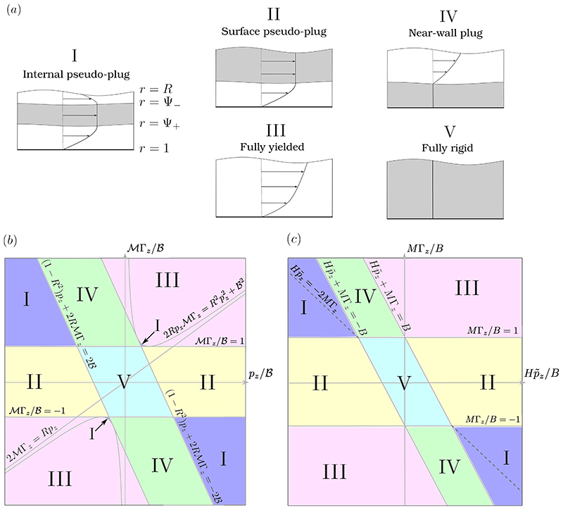
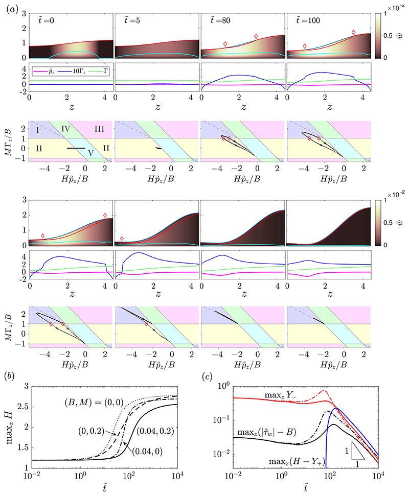
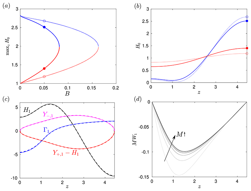
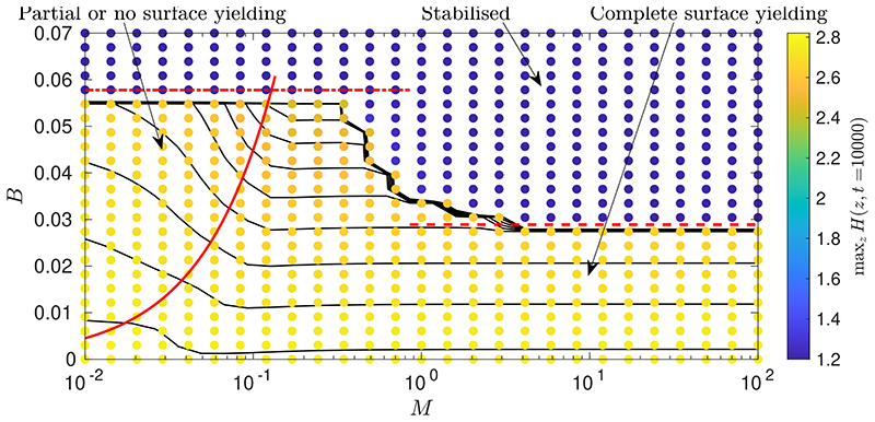
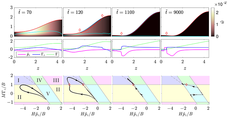
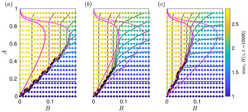
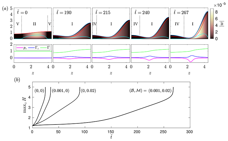
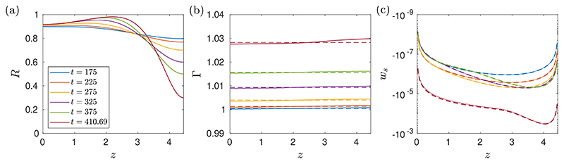
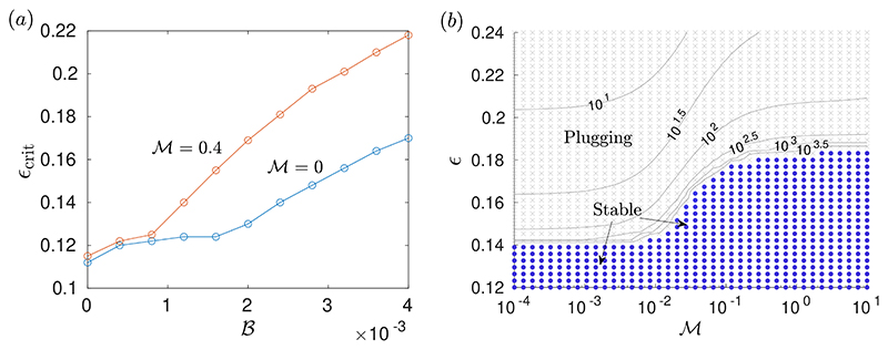
To assess how the presence of surfactant in lung airways alters the flow of mucus that leads to plug formation and airway closure, we investigate the effect of insoluble surfactant on the instability of a viscoplastic liquid coating the interior of a cylindrical tube. Evolution equations for the layer thickness using thin-film and long-wave approximations are derived that incorporate yield-stress effects and capillary and Marangoni forces. Using numerical simulations and asymptotic analysis of the thin-film system, we quantify how the presence of surfactant slows growth of the Rayleigh-Plateau instability, increases the size of initial perturbation required to trigger instability and decreases the final peak height of the layer. When the surfactant strength is large, the thin-film dynamics coincide with the dynamics of a surfactant-free layer but with time slowed by a factor of four and the capillary Bingham number, a parameter proportional to the yield stress, exactly doubled. By solving the long-wave equations numerically, we quantify how increasing surfactant strength can increase the critical layer thickness for plug formation to occur and delay plugging. The previously established effect of the yield stress in suppressing plug formation [Shemilt et al., J. Fluid Mech., 2022, vol. 944, A22] is shown to be amplified by introducing surfactant. We discuss the implications of these results for understanding the impact of surfactant deficiency and increased mucus yield stress in obstructive lung diseases.

Figure 1

Left: sketch of the model geometry. The air-liquid interface is located at r = R(z, t). Insoluble surfactant is present at the interface, with (non-dimensionalised) concentration Γ. Right: an illustration of a possible axial velocity profile in the liquid layer, w. Fully yielded, shear-dominated regions (white) are shown adjacent to the interface (R ⩽ r ⩽ Ψ₋) and adjacent to the wall (Ψ₊ ⩽ r ⩽ 1), with a plug-like region (grey) in between (Ψ₋ < r < Ψ₊).

Figure 2

(a) The fives types of yielding that can occur in the layer. Plug-like regions are shown in grey and fully-yielded regions in white. Typical axial velocity profiles are also sketched. Below are maps of parameter space showing where these yielding types occur in (b) the long-wave system and (c) the thin-film system. When plotting the map in (b), we treat R as a fixed parameter in order to focus on variation with p_z and 𝓜Γ_z. In (b), as in §2.3, the parameter map is plotted in terms of the unscaled variables (2.9). In (c), the map is plotted in terms of the scaled thin-film variables introduced in (2.37). Along the dashed line in (c), the surface velocity is exactly zero, ${\tilde{w}}_s=0$.

Figure 3

(a) Snapshots from a numerical solution of the thin-film evolution equations (2.40)-(2.45) with B = 0.04, M = 0.2, A = 0.2 at $\tilde{t}=\{0,5,80,100,130,250,500,2000\}$. At each $\tilde{t}$, there are three panels: the top panel shows the layer evolving, with Y₋ (cyan) and Y₊ (red), and the thin-film axial velocity $\tilde{w}$ represented by the colour map; the middle panel shows plots of ${\tilde{p}}_z$ (magenta), Γ (green) and 10Γ_z (blue); the bottom panel shows the solution in $\left(H{\tilde{p}}_z/B,M{\text{Γ}}_z/B\right)$-space, in dotted black lines, with the dots corresponding to points evenly spaced along the domain 0 < z < L and the arrows indicating the direction of increasing z. Red diamonds on the first and third panels mark the boundaries of the region where there is yielding at the interface. (b) Time evolution of max_z H from the same simulation (solid), compared to the evolution of max_z H from a Newtonian surfactant-laden simulation with (B, M) = (0,0.2) (dashed), a surfactant-free viscoplastic simulation with (B, M) = (0.04,0) (dot-dashed) and a surfactant-free Newtonian simulation with (B, M) = (0,0) (dotted). (c) Time evolution of max_z Y₋ (solid red), max_z(H − Y₊) (solid blue) and ${\max }_z\left(\left|{\tilde{\tau }}_w\right|-B\right)$ (solid black) for the simulation in (a). Also shown are plots of max_zY₋ (dot-dashed red) and ${\max }_z\left(\left|{\tilde{\tau }}_w\right|-B\right)$ (dot-dashed black) for the surfactant-free viscoplastic simulation (B = 0.04, M = 0).

Figure 4

(a) Plot of max_z H₀ for all the solutions to (3.2a) (solid), which are static, marginally-yielded solutions to the thin-film equations with surfactant. For comparison, the equivalent plot for the static solutions for the surfactant-free problem, which were computed in Shemilt et al. (2022), is also shown (dotted). The four coloured markers in (a) correspond to the example solutions shown in (b). All solutions in (b) have B = 0.05 but the dotted ones are the solutions for the surfactant-free problem. (c) O (1/t) terms in the late-time expansion (3.3) for a solution with B = 0.05 and M = 0.5, showing H₁ (solid black), Y_−,1 (solid magenta), Y_+,1, − H₁ (solid red) and Γ₁ (solid blue). These are compared to corresponding quantities from a numerical solutions of the thin-film equations 2.40)-(2.45 at $\tilde{t}={10}^4$, specifically $\left[H\left(z,\tilde{t}={10}^4\right)-H_0(z)\right]B\tilde{t}$ (dashed black), $Y_{-}\left(z,\tilde{t}={10}^4\right)B\tilde{t}$ (dashed magenta), $\left[Y_{+}\left(z,\tilde{t}={10}^4\right)-H\left(z,\tilde{t}={10}^4\right)\right]B\tilde{t}$ (dashed red) and $\left[\text{Γ}\left(z,\tilde{t}={10}^4\right)-{\text{Γ}}_0(z)\right]B\tilde{t}$ (dashed cyan) where Γ₀ is defined in (3.2b). (d) Leading-order surface velocity, W₁, scaled by M, for B = 0.05 and M = {0.25, 0.5, 1, 2, 4, 8}.

Figure 5

Data from thin-film simulations with A = 0.2 and various B and M. Each coloured point corresponds to one simulation with the colour indicating the final peak height. Contours interpolated from the same data are also plotted in black, which are evenly spaced and in the range 2.4 ⩽ max_z H ⩽ 2.8. The red lines are 2M = BL (solid), B = B_m(A = 0.2) ≈ 0.0289 (dashed) and B = 2B_m(A = 0.2) ≈ 0.0578 (dot-dashed).

Figure 6

Snapshots from a thin-film simulation with B = 0.04, M = 0.08, A = 0.2, at $\tilde{t}=\{70,120,1100,9000\}$. The upper row of panels shows the layer height evolving, with Y₋ (cyan) and Y₊ (red), and the thin-film axial velocity, $\tilde{w}$, represented by the colour map; the middle row shows Γ (green), Γ_z (blue) and ${\tilde{p}}_z$ (magenta); and the lower row shows shows the solution in $\left(H{\tilde{p}}_z/B,M{\text{Γ}}_z/B\right)$-space, with the black dots corresponding to evenly spaced points along 0 < z < L and the arrows indicating the direction of increasing z. Red diamonds on the first and third panels mark the boundaries of the region where there is yielding at the interface.

Figure 7

Data from thin-film numerical simulations with (a) M = 0, (b) M = 0.6 and (c) M = 6. Each coloured dot corresponds to one simulation, with the given values of A and B, where the colour indicates the final maximum height of the layer. The same data for max_z H(z, t = 10⁴) is linearly interpolated and plotted as black contour lines. The two magenta curves on each panel are B = B_m(A) (solid) and B = 2B_m(A) (dot-dashed).

Figure 8

(a) Numerical solution of the long-wave equations (2.25)-(2.33) with A = 0.2, 𝓑 = 0.001, 𝓜 = 0.02 and ϵ = 0.14, showing the transition towards plug formation. The upper panel shows the evolution of the layer height, with Y₋ (cyan) and Y₊ (red) also shown, and the colour corresponding to the magnitude of the axial velocity, |w|. The lower panel shows p_z (magenta), Γ_z (blue) and Γ (green). (b) Time evolution of max_z H for the same simulation, compared to max_zH from simulations with (𝓑, 𝓜) = {(0, 0), (0.001, 0), (0, 0.02), (0.001, 0.02)}, showing the combined delay to plug formation by surfactant and yield stress.

Figure 9

Results from a numerical solution of the long-wave equations with ϵ = 0.14, 𝓜 = 10, 𝓑 = 0.001 and A = 0.25. (a) The interface position, R, shown at various time points. The last time point is $\tilde{t}=t_p=410.69$, when the simulation is stopped. (b) Surfactant concentration, Γ, (solid) at the same time points as in (a). These are compared to 𝓖0 (t) (dashed), the approximation from the large-𝓜 asymptotic theory, which is evaluated via (4.2) using the numerical solutions from (a) as proxies for 𝓡₀. (c) Surface velocity, w_s, (solid) at the same time points. These are also compared to the corresponding approximation from the large-𝓜 theory (4.3).

Figure 10

(a) Critical layer thickness, ϵ_crit, as a function of 𝓑, for a surfactant-free layer (𝓜 = 0) and a layer with surfactant (𝓜 = 0.4). All simulations have A = 0.25. The value of ϵ_crit computed is such that a simulation with ϵ = ϵ_crit + 0.001 forms a plug before $\tilde{t}={10}^4$ and a simulation with ϵ = ϵ_crit − 0.001 has not formed a plug by $\tilde{t}={10}^4$. (b) Data from long-wave simulations at various values of ϵ and 𝓜, with A = 0.25 and 𝓑 = 0.0024. Grey crosses indicate simulations where a liquid plug formed, while black dots indicate simulations where a plug did not form. Within the plugging region, the grey contours indicate the plugging time, t_p.

References

1. Ahmadikhamsi S, Golfier F, Oltean C, Lefévre E, Bahrani SA. Impact of surfactant addition on non-newtonian fluid behavior during viscous fingering in hele-shaw cell. Phys Fluids. 2020;32(1):012103
1. Balmforth NJ, Craster RV. A consistent thin-layer theory for Bingham plastics. J Non-Newton Fluid Mech. 1999;84(1):65–81.
1. Balmforth NJ, Ghadge S, Myers TG. Surface tension driven fingering of a viscoplastic film. J Non-Newton Fluid Mech. 2007;142(1):143–149.
1. Billingham J, King AC. Wave Motion. Cambridge University Press; 2001.
1. Camassa R, Forest MG, Lee L, Ogrosky HR, Olander J. Ring waves as a mass transport mechanism in air-driven core-annular flows. Phys Rev E. 2012;86(6):066305 - PubMed
LinkOut - more resources