Revealing invisible cell phenotypes with conditional generative modeling

Abstract

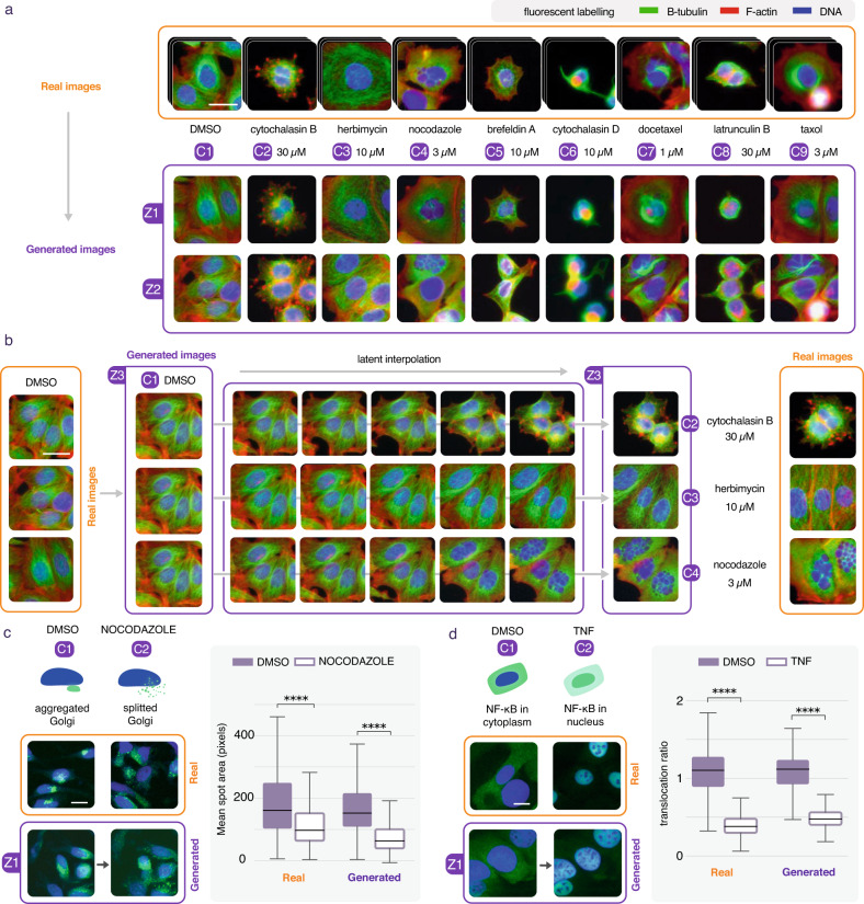
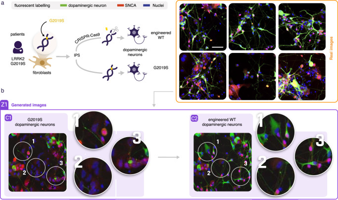
Biological sciences, drug discovery and medicine rely heavily on cell phenotype perturbation and microscope observation. However, most cellular phenotypic changes are subtle and thus hidden from us by natural cell variability: two cells in the same condition already look different. In this study, we show that conditional generative models can be used to transform an image of cells from any one condition to another, thus canceling cell variability. We visually and quantitatively validate that the principle of synthetic cell perturbation works on discernible cases. We then illustrate its effectiveness in displaying otherwise invisible cell phenotypes triggered by blood cells under parasite infection, or by the presence of a disease-causing pathological mutation in differentiated neurons derived from iPSCs, or by low concentration drug treatments. The proposed approach, easy to use and robust, opens the door to more accessible discovery of biological and disease biomarkers.

Fig. 1. Conditional synthesis of cell phenotype perturbations.

a A conditional GAN is trained on real images (orange) of DMSO and high concentration drug treatments (C1, C2, C3, etc.), scale bar is 20 μm. Synthetic images (violet) of these treatments can be generated from the same random seed, here z1 or z2. The high compound concentrations of these examples make the phenotypic changes obvious and visible. Surrounding cells in the negative control (DMSO) are removed from the images of compound treatments because of their toxicity. b A latent traversal can be computed for a single seed (z3) from the untreated state (C1 = DMSO) to 3 different treatment effects (C2,C3,C4) displaying each a different gradual change of the same cells. c A standard assay such as the nocodazole induced golgi scattering (green) can be reproduced with synthetic images, scale bar is 20 μm. An image analysis measurement (mean spot area) performed on real and synthetic images of both conditions led to the same quantitative conclusion (n = 1000 for each sampled condition, two sided t-test. Real: p = 5.1e-19, T(1998) = 9.0, confidence interval(99.99%) = [43.05, 108.84], Cohen’s d = 0.403. Generated: p = 5.35e-113, T(1998) = 24.12, Confidence interval(99.99%) = [78.0, 108.02] Cohen’s d = 1.079, ****p-value < 0.0001). d Another standard assay displaying TNF-induced NFkB translocation (green) can also be reproduced, scale bar is 20 μm (n = 1000 for each sampled condition, two sided t-test. Real: p = 0, T(1998) = 178.2, Confidence interval(99.99%) = [0.66, 0.69], Cohen’s d = 2.87. Generated: p = 0, T(1998) = 60.73, Confidence interval(99.99%) = [0.53, 0.60], Cohen’s d = 2.75, ****p-value < 0.0001), p values were not adjusted. Boxes represent the q1-q3 interval (25–75% of the distribution). The central bar is the median. The lower whisker is the first datum greater than q1 − 1.5 × IQR and the upper whisker is the last datum lower than q3 + 1.5 × IQR. IQR is interquartile range. Source data are provided as a Source Data file.

Fig. 2. Unraveling red blood cell morphological changes related to an infectious environment.

a Images of blood cells were extracted from thin blood smears sampled from a population of people exposed to malaria. In all, 200 slides were selected as negative for Malaria by microscopists, meaning that no parasites could be found on any of these slides, with nevertheless half of them found to be positive by qPCR. Note that on both qPCR positive and qPCR negative slides, images extracted displayed variable cell densities with variable background, did not contain any parasites, and did not show any identifiable systematic visible differences, scale bar is 10 μm. b In order to identify discriminative features between qPCR+ and qPCR- slides, we used 60,000 such images from these 200 slides to train a conditional GAN. This panel shows three representative generated images of the results found. Z1 displays a visual difference that can be interpreted as an increase of anemia: the content of some blood cells lose hemoglobin (displayed as a hole or a white halo in the cell). This phenotype could barely be identified from real images data because both qPCR+ and qPCR- slides contain anemia cells. Additionally, Z2 displays some deformations of the cell membrane producing crenated cells. Finally, Z3 shows that the negative sample contained more debris due to staining as a translation to qPCR+ tends to remove these artifacts. Indeed, the system cannot discriminate between relevant differences of phenotypes from biologically irrelevant differences related to possible technical or experimental biases.

Fig. 3. Unraveling invisible morphological variation in a patient-derived dopaminergic neuron assay.

a IPSCs are derived from fibroblasts sampled from a LRRK2 G2019S mutated Parkinson’s patient. These IPScs are then reprogrammed to dopaminergic neurons with or without a CRISPR-cas9 correction of the G2019S mutation. The latter is an isogenic engineered wild type. Large sets of confocal images with one dye labeling for Nuclei, and antibody stains labeling for alpha-synuclein and TH cells, scale bar is 20 μm. Real images display no detectable visual systematic differences. b A conditional GAN trained in order to identify differences between these two close conditions displays 1 - an increase of dopaminergic neurons and dendritic complexity in the engineered WT condition, 2 - removal of some of the IPScs in the WT condition, 3- alpha-synuclein seems to shift from the IPSc cytoplasm to the nuclei before it eventually decreases in fully shaped differentiated WT neurons (more examples here https://www.phenexplain.bio.ens.psl.eu/lrrk2.html).

Fig. 4. Morphological effect of perturbations by low dose compound treatments and dose response.

a The same compounds used at high concentration in Fig. 1 were also plated at very low concentrations. The corresponding images cannot be visually distinguished from untreated cells (DMSO) and from one another (first row), scale bar is 20 μm. A conditional GAN was trained on real images of these low concentration compound treatments. By doing so we could generate artificial images of these perturbations on the same cells and compare them with DMSO and with each other (second row). We see that most treatments, even at low doses, had a slight toxic effect as they removed cells on the image borders compared to DMSO. Furthermore, some compounds tend to expand the cell cytoplasm while some others contract it. b An LDA plan is computed from generation of 3000 DMSO, 3000 Nocodazole and 3000 cytochalasin B at highest doses. Then, 300 samples of each available concentration of the Nocodazole treatment were drawn and projected onto this plan. c Left column, real images from a nocodazole dose response, middle column, z2 is a random seed used to generate perturbations of the same cells for each concentration (green dots on panel b) and, right column represents their orthogonal projections on the latent traversal between DMSO and the highest nocodazole dose in the W space: red dots on the red axis. d Computation of the distances in the W space of n = 1000 samples from each dose (C2, C3, etc.) to the DMSO (C1) for a given compound enables construction of a dose response curve describing the gradual intensity of the morphological changes. Boxes represent the q1-q3 interval (25–75% of the distribution). The central bar is the median. The lower whisker is the first datum greater than q1 − 1.5 × IQR and the upper whisker is the last datum lower than q3 + 1.5 × IQR. Source data are provided as a Source Data file.

References

1. Lundervold AS, Lundervold A. An overview of deep learning in medical imaging focusing on MRI. Z. Med. Phys. 2019;29:102–127. doi: 10.1016/j.zemedi.2018.11.002. - DOI - PubMed
1. Moen E, et al. Deep learning for cellular image analysis. Nat. Methods. 2019;16:1233–1246. doi: 10.1038/s41592-019-0403-1. - DOI - PMC - PubMed
1. Ching, T. et al. Opportunities and obstacles for deep learning in biology and medicine. J. R. Soc. Interface15, 20170387 (2018). - PMC - PubMed
1. van der Walt S, et al. scikit-image: image processing in Python. PeerJ. 2014;2:e453. doi: 10.7717/peerj.453. - DOI - PMC - PubMed
1. Carpenter AE, et al. CellProfiler: image analysis software for identifying and quantifying cell phenotypes. Genome Biol. 2006;7:R100. doi: 10.1186/gb-2006-7-10-r100. - DOI - PMC - PubMed
Publication types
LinkOut - more resources