Synchronizing chaos using reservoir computing

Abstract

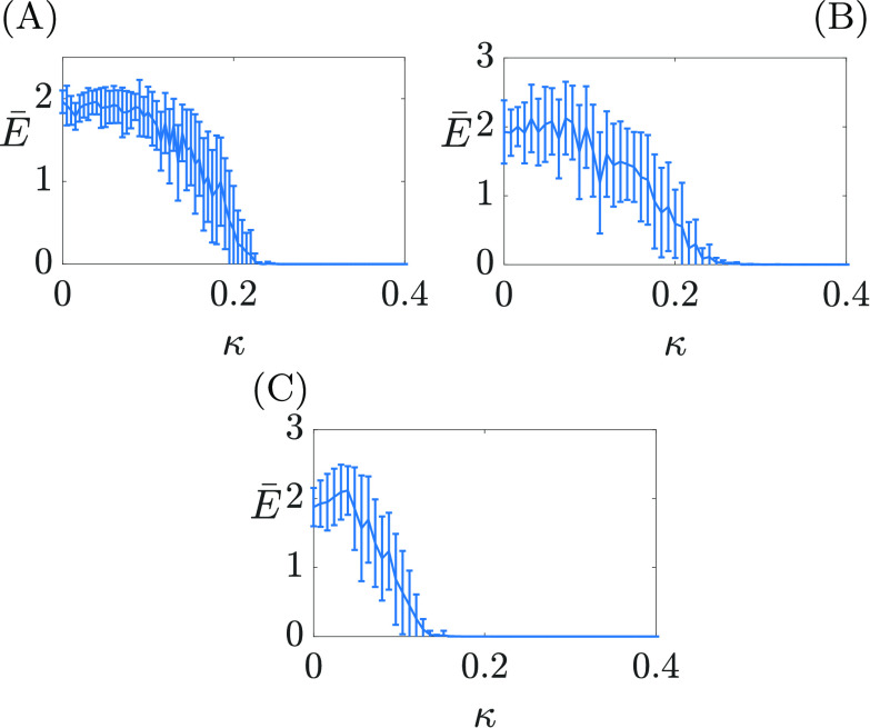
We attempt to achieve complete synchronization between a drive system unidirectionally coupled with a response system, under the assumption that limited knowledge on the states of the drive is available at the response. Machine-learning techniques have been previously implemented to estimate the states of a dynamical system from limited measurements. We consider situations in which knowledge of the non-measurable states of the drive system is needed in order for the response system to synchronize with the drive. We use a reservoir computer to estimate the non-measurable states of the drive system from its measured states and then employ these measured states to achieve complete synchronization of the response system with the drive.

FIG. 1.

(a) Training phase of reservoir. The reservoir input signal is $x_D(t)$, and it is trained on $y_D(t)$. The error, $E(t)$, is calculated with the fit signal, $\hat{y}(t)$, and the training signal. (b) Control configuration. The response system takes as an input, $\mathit{E}(t)$, where $\mathit{E}(t)=H({\mathit{v}}_R(t)-{\mathit{v}}_D(t))$. The matrix, $H$, describes what state variables are used in the coupling. I/R is the input to reservoir function and R/O is the output to reservoir function.

FIG. 2.

Chen system. (a) Coupled $x_D\to y_R$, ${\kappa }_{min}\simeq 10.78$. (b) Coupled ${\hat{y}}_D\to y_R,{\kappa }_{min}\simeq 3.96$. (c) Coupled both $x_D\to y_R$ and ${\hat{y}}_D\to y_R,{\kappa }_{min}\simeq 3.00$. The error bars represent standard deviations over 20 realizations.

FIG. 3.

The plots show the time evolution of the $x$ component of the drive and the response systems when coupled through the RC in $x_D\to y_R$ and ${\hat{y}}_D\to y_R$ (top) and when coupled ideally in $x_D\to y_R$ and $y_D\to y_R$ (bottom). Here, the coupling strength $\kappa =3.1$ for both cases.

FIG. 4.

Synchronization error of Chen’s drive and response systems from time series in Fig. 3. The plot shows $E_{\mathrm{RC}}(t)$, the error when the coupling $x_D\to y_R$ and ${\hat{y}}_D\to y_R$ is through estimation by RC, and $E_{\mathrm{Ideal}}(t)$, the error in the ideal case when both states of the drive system are known, $x_D\to y_R$ and $y_D\to y_R$.

FIG. 5.

The absolute difference between the estimated driver signal ${\hat{y}}_D(t)$ and the true signal $y_D(t)$.

FIG. 6.

Chen system. Coupling is in $x_D\to x_R$ and ${\hat{y}}_D\to y_R$ with $\kappa =10$. (a) We plot the training ${\mathrm{\Delta }}_{\mathrm{tr}}$, testing ${\mathrm{\Delta }}_{\mathrm{ts}}$, and synchronization $E$ errors as a function of the leakage parameter, $\alpha$ for a fixed value of the spectral radius $\rho =0.9$. (b) We plot the training, testing, and synchronization error as a function of the spectral radius, $\rho$, of the $A$ matrix, for a fixed value of the leakage parameter $\alpha =0.5$.

FIG. 7.

Rössler system. Coupling is in $x_D\to x_R$ and ${\hat{y}}_D\to y_R$ with $\kappa =0.15$. (a) We plot the training, testing, and synchronization error as a function of the leakage parameter, $\alpha$. We set $\rho =0.6$ (b) We plot the training, testing, and synchronization error as a function of the spectral radius, $\rho$ of the $A$ matrix, for a fixed value of the leakage $\alpha =0.05$.

FIG. 8.

Rössler system. (a) Coupling $x_D\to x_R$. (b) Coupling ${\hat{y}}_D\to y_R$. (c) Coupling is both $x_D\to x_R$ and ${\hat{y}}_D\to y_R$. The error bars represent the standard deviations over 20 realizations.

FIG. 9.

Time trajectories of the $x$ components of the drive and the response systems when the drive Rössler system evolves on an unstable periodic orbit. In (a), the two systems are coupled with $x_D\to x_R$ with the coupling strength $\kappa =0.3$. In (b), the two systems are coupled with $x_D\to x_R$ and ${\hat{y}}_D\to y_R$ with the same $\kappa =0.3$. The estimation ${\hat{y}}_D$ is done through a reservoir computer, as explained in the text.

FIG. 10.

Rössler system. We plot the synchronization error as a function of the magnitude of noise, $ϵ$, as seen in Eq. (14). (a) compares the case of coupling ${\tilde{y}}_D\to y_R$ (noise corrupted) with the case ${\hat{y}}_D\to y_R$ (noise corrupted + RC). (b) compares the case of coupling ${\tilde{y}}_D\to y_R$ and ${\tilde{x}}_D\to x_R$ (noise corrupted) with the case ${\hat{y}}_D\to y_R$ and ${\tilde{x}}_D\to x_R$ (noise corrupted+RC). Here, the training and testing errors are ${\mathrm{\Delta }}_{\text{tr}}=1.14({10}^{-4})$, and ${\mathrm{\Delta }}_{\text{ts}}=1.45({10}^{-4})$ when $ϵ=0$.

References

1. Aranson I. and Rul’kov N., “Nontrivial structure of synchronization zones in multidimensional systems,” Phys. Lett. A 139(8), 375–378 (1989). 10.1016/0375-9601(89)90581-1 - DOI
1. Pikovskii A. S., “Synchronization and stochastization of array of self-excited oscillators by external noise,” Radiophys. Quantum Electron. 27(5), 390–395 (1984). 10.1007/BF01044784 - DOI
1. Fujisaka H. and Yamada T., “Stability theory of synchronized motion in coupled-oscillator systems,” Prog. Theor. Phys. 69(1), 32–47 (1983). 10.1143/PTP.69.32 - DOI
1. Afraimovich V. S., Verichev N. N., and Rabinovich M. I., “Stochastic synchronization of oscillations in dissipative systems,” Radiophys. Quantum Electron. 29, 795–803 (1986).10.1007/BF01034476 - DOI
1. Pecora L. M. and Carroll T. L., “Synchronization in chaotic systems,” Phys. Rev. Lett. 64(8), 821 (1990). 10.1103/PhysRevLett.64.821 - DOI - PubMed
LinkOut - more resources