. 2023 Oct 10:11:e16083.
doi: 10.7717/peerj.16083. eCollection 2023.

Dynamic analysis and control of a rice-pest system under transcritical bifurcations

Affiliations

Dynamic analysis and control of a rice-pest system under transcritical bifurcations

Sajib Mandal et al. PeerJ. .

Abstract

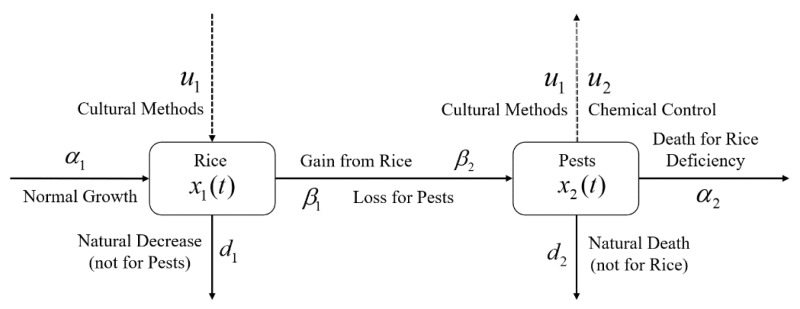
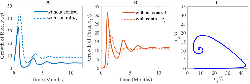
A decision model is developed by adopting two control techniques, combining cultural methods and pesticides in a hybrid approach. To control the adverse effects in the long term and to be able to evaluate the extensive use of pesticides on the environment and nearby ecosystems, the novel decision model assumes the use of pesticides only in an emergency situation. We, therefore, formulate a rice-pest-control model by rigorously modelling a rice-pest system and including the decision model and control techniques. The model is then extended to become an optimal control system with an objective function that minimizes the annual losses of rice by controlling insect pest infestations and simultaneously reduce the adverse impacts of pesticides on the environment and nearby ecosystems. This rice-pest-control model is verified by analysis, obtains the necessary conditions for optimality, and confirms our main results numerically. The rice-pest system is verified by stability analysis at equilibrium points and shows transcritical bifurcations indicative of acceptable thresholds for insect pests to demonstrate the pest control strategy.

Keywords: Decision model; Integrated pest management; Lotka-Volterra model; Nonlinear dynamics; Optimal control; Predator-prey.


Conflict of interest statement

The authors declare there are no competing interests.

Figures

Figure 1
Figure 1. Annual production and losses of rice from 1960–2013 and the most common factors responsible for the rapid increase in annual global losses of rice over the years.
(Left) Annual production and losses of rice from 1960–2013 (FAO, 2021) represented under a logarithmic scale with MMT measurement unit. In comparison to production, annual losses increased over the years and their absolute number is very high, and (right) the most common factors responsible for the rapid increase in annual global losses of rice over the years. The increasing density of pests and excessive use of pesticides in paddy fields are the major causes of the losses of rice. Only the factors identified in red frames are considered in this study.
Figure 2
Figure 2. A decision-making diagram of the decision model Eq. (4) that describes the ideal timing for the application of pesticides.
Here, D = 1 represents the acceptable damage threshold reaching a maximum of still acceptable pollution. AT denotes the action threshold to determine the use of pesticides to control the pest population, and ACT represents the interval in which pesticides should be applied. When the density of the pest population crosses the AT line, pesticides are applied. Due to the use of pesticides, the growth rate of pests gradually slows down. When the pesticides are used at full scale (u2 =1), the growth rate of pests starts decreasing after reaching a stable situation. Because u2 = 1, the acceptable damage threshold reaches the maximum level i.e., D = 1; the use of pesticides is stopped (u2 = 0) to limit the environmental pollution (defined in the 4th row of Eq. (4)).
Figure 3
Figure 3. Schematic diagram of the rice-pest-control system Eq. (7) describes the rice-pest system (S4) under control.
The diagram also shows that the control strategies, cultural methods and chemical control (pesticides), increase rice production and reduce corresponding pest populations.
Figure 4
Figure 4. Time series and phase portrait of the rice-pest system (S4).
(A) Time series of annual rice production and rice pest population and (B) phase portrait of the rice-pest system (S4) with the solution (4.12, 11.54).
Figure 5
Figure 5. Time series of (A) annual rice production, and (B) rice pest population for different consumption rates of the pests.
Figure 6
Figure 6. Time series of the annual production of rice and pest population when only cultural methods are adopted as a control strategy.
Time series of (A) annual rice production under control u1 only, (B) pest population under control u1 only, (C) phase portrait of the rice-pest-control system Eq. (7) when only u1 is adopted, where the solution is (8.81, 10.79).
Figure 7
Figure 7. Time series of the annual production of rice and pest population when only chemical controls are adopted as a control strategy.
Time series of (A) annual production of rice under control u2 only, (B) pest population under control u2 only, (C) phase portrait of the rice-pest-control system Eq. (7) when only u2 is adopted and the solution is (12.86, 9.17).
Figure 8
Figure 8. Time series of the annual production of rice and pest population when both controls, cultural methods and chemical controls are implemented.
Time series of (A) annual production of rice under controls u1 and u2, (B) pest population under u1 and u2, (C) phase portrait of the rice-pest-control system Eq. (7) when both u1 and u2 are implemented, where the solution is (19.18, 7.73).
Figure 9
Figure 9. A comparison between scenarios (i) to (iii).
Here, (A) The time series of the annual production of rice; (B) the time series of pest populations under three different scenarios.
Figure 10
Figure 10. Diagram for the isocline of the rice (vertical) and the pest’s isocline (inclined)
(A) β = 0.8; (B) β = 1; (C) β = 2, where α = 1 and γ = 0.001 remains same.
Figure 11
Figure 11. Phase plane describing the nature of the rice-pest system (S16) at the interior point for the variation of bifurcation parameter (β)
(A) β = 2, (B) β = 10.9, (C) β = 11.1, (D) β = 12, (E) β = 12.66, and (F) β = 13.6, where α = 1 and γ = 0.001 remain same.
Figure 12
Figure 12. Transcritical bifurcation diagram of the rice-pest system (S16) for the bifurcation parameter showing whether the system is stable, limit cycle and unstable.
The bifurcation diagram shows that the system (S16) is stable for β from 1 to 11, experiences limit cycle for β from 11.1 to 13.6, and unstable for β from 0 to <1 and for >13.6. The figure reveals that the rice-pest system (S16) is present within the acceptable thresholds of the pests population and is destroyed above and below the acceptable thresholds.

Similar articles

References

    1. Alphey M, Bonsall MB. Genetics-based methods for agricultural insect pest management. Agricultural and Forest Entomololy. 2018;20(2):131–140. doi: 10.1111/afe.12241. - DOI - PMC - PubMed
    1. Banerjee M, Petrovskii S. Self-organised spatial patterns and chaos in a ratio-dependent predator—prey system. Theoretical Ecology. 2011;4(1):37–53. doi: 10.1007/s12080-010-0073-1. - DOI
    1. Bazykin AD. Structural and dynamic stability of model predator-prey systems. International Institute for Applied Systems Analysis (IIASA) Research Memorandum; Laxenburg, Austria: 1976.
    1. Benett J, Bentur JC, Pasula IC, Krishnaiah K. New approaches to gall midge resistance in rice. New Delhi: International Rice Research Institute and Indian Council of Agricultural Research; 2004.
    1. Bhattacharyya S, Bhattacharya DK. Pest control through viral disease: mathematical modeling and analysis. Journal of Theoretical Biology. 2006;238(1):177–197. doi: 10.1016/j.jtbi.2005.05.019. - DOI - PubMed