The rat frontal orienting field dynamically encodes value for economic decisions under risk

Abstract

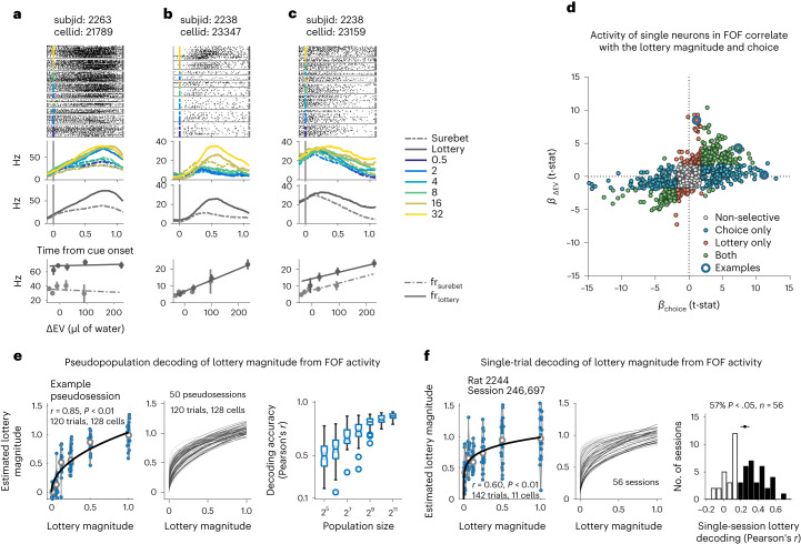
Frontal and parietal cortex are implicated in economic decision-making, but their causal roles are untested. Here we silenced the frontal orienting field (FOF) and posterior parietal cortex (PPC) while rats chose between a cued lottery and a small stable surebet. PPC inactivations produced minimal short-lived effects. FOF inactivations reliably reduced lottery choices. A mixed-agent model of choice indicated that silencing the FOF caused a change in the curvature of the rats' utility function (U = V^ρ). Consistent with this finding, single-neuron and population analyses of neural activity confirmed that the FOF encodes the lottery value on each trial. A dynamical model, which accounts for electrophysiological and silencing results, suggests that the FOF represents the current lottery value to compare against the remembered surebet value. These results demonstrate that the FOF is a critical node in the neural circuit for the dynamic representation of action values for choice under risk.

Fig. 1. The task and animal behavior.

a, Schematic of the task. On each trial, rats initiated the trial by fixating in the center port. At the onset of fixation, a tone was played, indicating the magnitude of the lottery. The tone remained on until the response in the choice port (see Methods for details). b, An example sequence of trials. For trial type, white diamonds, yellow triangles and blue triangles represent choice trials, forced lottery trials and forced surebet trials, respectively. The sine waves in the ‘tone freq’ illustrate that the lottery sound varied from trial to trial. Animalsʼ responses are marked in diamonds, with yellow for lottery and blue for surebet. The reward received (μl) on each trial is shown in light blue circles, whose size represents the relative amount. The red cross indicates a ‘lottery-lose’ trial. c, Example subject performance from rat 2154 (from the muscimol experiments). The probability of choosing lottery is plotted as a function of the EV of lottery minus the EV of surebet in μl of water. The circles with error bars are the mean and 95% binomial CIs. The lines are psychometric curves generated by a logistic fit; the thin gray lines are fits to each session; and the thick gray line is the fit to all the sessions combined (n = 1,135 trials, 16 sessions). d, Subject performance from control sessions for all experiments. For muscimol animals, control sessions were 1 d before an infusion event. For optogenetic animals, we include the control trials from sessions with laser stimulation. The lines are logistic fits from each animal, with the color of the line indicating the experiment that animal participated in (n =33,511 trials, 319 sessions, 8 rats for infusion, 8 rats for optogenetics and 6 rats for electrophysiology).

Fig. 2. Effects of silencing PPC and FOF.

a, Top-down view of the rat cortex with the target coordinates of FOF and PPC, where the cannulae or optical fibers were implanted. b–g, Probability of choosing the lottery given the difference in the EV of the lottery and the surebet. The circles with error bars are the mean and 95% binomial CIs. Points are jittered to avoid visual overlap of error bars. The ribbons are from a logistic fit to the data. The number of trials indicated on each panel are the infusion trials only. For panels showing data from muscimol experiments, the control data are from 1 d before any infusion. For panels with optogenetic (opto) silencing, the control data are the no-laser trials in the same sessions. Significance (one-sided, *P < 0.05, **P < 0.005, ***P < 0.0005) was based on an LR test between a mixed-effect model with and without a variable indicating which sessions (or trials) were drug/laser versus control. See the statistical appendix for details. b, Bilateral PPC infusions. Control sessions are in gray (n = 24 sessions, 7 rats), and 0.3 μg per side bilateral PPC infusions (n = 12 sessions, 7 rats) are in yellow (LR test, χ²(2, N = 9,501) = 3.15, P = 0.21). c, Bilateral FOF infusions. Control sessions are in gray (n = 17 sessions, 8 rats); 0.075 μg per side bilateral FOF infusions (n = 6 sessions, 5 rats) are in pink; and 0.3 μg per side bilateral FOF infusions (n = 9 sessions, 8 rats) are in purple (LR test, χ²(2, N = 9,389) = 16.43, P = 2.7 × 10⁻⁴). d, Bilateral optogenetic silencing of the FOF. Control trials are in gray, and opto silencing trials are in purple (n = 29 sessions, 5 rats, LR test, χ²(2, N = 3,085) = 11.42, P = 3.3 × 10⁻³). e, Unilateral PPC infusions. Control sessions (n = 100 sessions, 8 rats) are in gray, and 0.3 μg PPC infusions (n = 31 sessions, 8 rats) are in pink (LR test, χ²(2, N = 11,110) = 3.67, P = 0.16). f, Unilateral FOF infusions. Control sessions (n = 39 sessions, 8 rats) are in gray, and 0.3 μg unilateral FOF infusion sessions (n = 36 sessions, 8 rats) are in pink (LR test, χ²(2, N = 10,866) = 13.52, P = 1.2 × 10⁻³). g, Unilateral optogenetic silencing of the FOF (left FOF n = 75 sessions, 8 rats; right FOF n = 51 sessions, 7 rats; LR test, χ²(2, N = 13,080) = 25.84, P = 2.4 × 10⁻⁶). h–j, These panels contain the same data as e–g but are re-organized to show possible ipsi-contra biases. The x axes are the EV of the right option versus the EV of the left option; the y axes are the probability of choosing the right option. If unilateral silencing produced contralateral neglect, then we would expect the psychometric curves from right infusions (in brown) to be above the left infusions (in dark blue) (h: n = 100 control sessions, 12 sessions for left PPC, 19 sessions for right PPC, 8 rats. LR test, χ²(1, N = 2,645) = 1.18, P = 0.28. i: n = 100 control sessions, 16 sessions for left FOF, 20 sessions for right FOF, 8 rats. LR test, χ²(1, N = 2,401) = 6.63, P = 0.01. j: n = 75 sessions for left FOF, 51 sessions for right FOF, 8 rats. LR test, χ²(1, N = 4,658) = 4.59, P = 0.03).

Fig. 3. FOF inactivation reduced the exponent of the utility function.

a, The three-agent model of risky choice. b, Psychometric curves from two example animals. The circles with error bars are the binned mean and 95% binomial CIs. The ribbons are model predictions generated using the fitted parameters (control, gray; bilateral FOF inactivation, purple). The solid line represents the model-predicted probability of lottery choice, and the dark and light shades represent 50% and 80% CIs, respectively. Similar plots for all animals are shown in Extended Data Figs. 3 and 4 (n = 801 control trials and 417 opto trials for rat 2228; n = 782 control trials and 73 infusion trials for rat 2160). c, Posterior distributions of changes in model parameters due to FOF silencing. An asterisk indicates that 97.5% of the posterior was not overlapping with 0. Silencing FOF consistently increased risk aversion through reducing the curvature of the utility function, ρ.

Fig. 4. Dynamical model of FOF silencing.

a, We implemented a six-node rate model of a distributed action value network with random connectivity ($W_{ij}~\mathcal{N}\left(5/6,1\right)$). The FOF was one of the six nodes (in purple). The input to the network was the lottery magnitude. b, Example of the network response to lottery sound with magnitude of 96 μl under control conditions (with all the nodes active, in gray) and under FOF silencing (the FOF node is set to zero, in purple). The dark traces represent the mean network activity, and the light traces represent the activity of the six individual nodes. c, Silencing FOF scales down the representation of the action value of the lottery, which could explain the shift in ρ. We ran the network for 20 ‘trials’ of each lottery ∈ [0, 12, 24, 48, 96, 192] μl. The gray circles are the mean and 95% CI for the network response in the control conditions, and the purple diamonds are the mean and 95% CI for the network response when the FOF node is silenced. Fitting a power law utility function (U = V^ρ) to the network activity gives ρ ≈ 0.76 for control and ρ ≈ 0.6 after FOF silencing. The thin lines are power law utility functions that approximate the transformation from units of reward (μl) to utils in spikes per second. d, Behavioral effects of the FOF silencing in c. The scaling of activity results in a stimulus-dependent shift, quantitatively similar to our experimental observations.

Fig. 5. Neural activity in the FOF encoded lottery value and upcoming choice action during the fixation period.

a–c, Example neurons. Spike raster plots and PSTHs of three representative neurons show heterogeneous dynamics during the fixation period. The rasters and PSTHs were aligned to the lottery cue onset and sorted by different lottery cues (indicated by different color) and upcoming choices (solid line for lottery choices, dashed line for surebet choices). The lower PSTH was sorted only on the basis of upcoming choices. The bottom row (firing rate versus ΔEV) summarizes the relationship among the neural activity, lottery value and choice. The lines are fits of a linear model (Hz ~ ΔEV * choice) to the data (dots with error bars represent mean ± s.e.m.; a: n = 150 trials, b: n = 106 trials, c: n = 104 trials). d, Distribution of coefficients of the choice against ΔEV from the mixed-effects linear models to characterize the individual neuronal responses to upcoming choices or lottery values. Of 1,690 recorded neurons, 23.5% (n = 393) were tuned for upcoming choice alone; 6.8% (n = 114) were tuned purely for the lottery values; and 18.3% (n = 309) were tuned for both. Blue circled data show where the three example neurons are located in the scatter plot. e,f, Pseudopopulation (e) and single-trial decoding (f) of lottery magnitude from FOF neural activities. Left panels show the examples of pseudosession and single session. The violins with the dot plots show the correlation between the cross-validated linear-model-estimated lottery magnitudes and the original lottery magnitudes (normalized for each session to the maximum magnitude). The solid lines are fits of a power law model $\widehat{L}=\alpha L^r$, where the L is the normalized original lottery magnitudes, and $\widehat{L}$ is the linear-model-estimated lottery magnitudes. Here, r captures the nonlinear relationship between the original and estimated lottery magnitude (e: for the example pseudosession, the Pearson’s correlation between the true value and power-law-model-estimated value, n = 120 trials from 128 cells r = 0.85, P = 5.5 × 10⁻³⁶, two-sided, not adjusting for multiple comparisons. f: for the example session, the Pearson’s correlation between the true value and power-law-model-estimated value, n = 142 trials from 11 cells, r = 0.60, P = 7.6 × 10⁻¹⁵, two-sided, not adjusting for multiple comparisons). Middle panels show the power law fits for all pseudosessions with 128 cells and single sessions. The darkness of the lines show the scale of correlation between the original lottery magnitude and power-law-model-estimated ones (e: n = 50 pseudosessions, f: n = 56 sessions). Right panels shows the decoding accuracy for pseudopopulation and single-session decoding (e: n = 50 pseudosessions; the box-and-whisker plots show the median, lower/upper quartile, minimum/maximum and the outliers of the data, and the notch shows $median\pm \left(1.57\times interquartilerange\right)/\sqrt{n}$. f: n = 56 sessions; black bins indicate sessions that show significant decoding (Pearson’s correlation between the true value and power-law-model-estimated ones, P < 0.05). Black dot and bar above the histogram show the 95% CI of the mean).

Fig. 6. Infusions in PPC during surebet value change and free choice.

a, Schematic showing that changing the surebet magnitude is equivalent to shifting the choice boundary. The data points were simulated from a risk-neutral agent using the three-agent model (ρ = 1, σ = 3, ω_rational = 1). A smaller surebet magnitude (light blue) horizontally shifts the psychometric curve leftwards; a larger surebet magnitude (dark blue) shifts the curve rightwards. The frequency-to-lottery mapping remains the same. b, Changing surebet magnitude from 6.8 to 3 shifted choices leftwards in one example animal. Combined trials from six sessions before the change are shown in gray, after the change shown in blue. One three-agent model was fit to all the trials, and the parameters were used for ribbon extrapolation (n = 547 trials for surebet magnitude is 6.8; n = 585 trials for surebet magnitude is 3; the circles with error bars are the mean and 95% binomial CIs). c, Same as b but with 0.6 μg per side bilateral PPC infusion, performed on the day of surebet change (from 3 to 6.8—n = 585 trials for surebet value is 3; n = 503 trials for surebet value is 6.8; the circles with error bars are the mean and 95% binomial CIs). d, The three-agent mixture model predicts the shifts in behavior well. One model was fit using all the sessions containing various surebet magnitudes for each animal. On the x axis is the predicted shift in probability choosing lottery: the difference in P(Choose Lottery) between model prediction using the new surebet magnitude and the session just before that change. On the y axis is the actual shift in P(Choose Lottery): the difference in P(Choose Lottery) between the first session of a surebet change and the session before that change. Sessions with just surebet change are in blue (n = 21, 4 animals); sessions with both surebet change and 0.6 μg per side bilateral PPC infusions are in gold (n = 8). There is a strong correlation between predicted and actual shift (Pearson’s correlation, r = 0.905, P = 1.6 × 10⁻¹¹), and this relationship is significantly different between shifts where PPC was silenced and control shifts (LR test, χ²(2, 29) = 7.44, P = 6.4 × 10⁻³). e, Schematic of the free trials. After fixation at the center port accompanied by a neutral tone, the animal was free to choose the left or right port, both illuminated in blue LEDs. Choosing either port resulted in a reward twice the magnitude of surebet. The free trials were randomly interleaved with the forced and choice trials. f, Unilateral PPC infusions (0.6 μg) led to a significant ipsilateral bias toward the side of infusion. This panel shows % ipsilateral bias: (∑choose_infusion_side − ∑choose_other_side) / ∑total_choices, when the side of infusions was chosen to be the opposite to the animalsʼ preferred side. % ipsilateral bias was computed using free trials from the previous three sessions, the infusion session and the following three sessions for six subjects. g, Left: unilateral PPC infusions generated a significant 52 ± 16% (t(5) = 3.09, P = 0.027, mean ± s.e. across rats, n = 6, two-sided) change in % ipsilateral bias on free trials compared to control sessions (three pre-infusion sessions). For the choice trials from the same sessions, the change in % ipsilateral bias was not significant (15 ± 8%, t(5) = 1.92, P = 0.11, mean ± s.e. across rats, n = 6, two-sided). Right: performance on the choice trials was not affected. Control sessions from the three pre-infusion sessions (n = 65 sessions, 6 rats) are in gray; 0.6 μg left PPC infusions (n = 5 sessions) are in blue; and 0.6 μg right PPC infusions (n = 6 sessions) are in orange.

Extended Data Fig. 1. Timeline of the risky-choice task and the relationship between utility curvature and risk aversion.

a. Illustration of the timeline of a risky-choice trial. b. The relationship between utility curvature and risk aversion. Consider a subject with a concave utility function, U = V^0.55. They are offered a choice between a surebet of 10 dollars or a 50/50 lottery that pays out 25 dollars or nothing. The green line indicates the utility of the surebet U_SB = 10^0.55 ≈ 3.55. The red dashed line connects the two possible outcomes of the lottery, 0^0.55 = 0 and 25^0.55 ≈ 5.87. The expected utility of the lottery is the weighted sum of the offers, U_L = 0.5 ⋅ 0 + 0.5 ⋅ 5.87 = 2.94. Since U_L < U_SB the subject will choose the surebet. If this lottery was offered 100 times, the subject would have 1000 dollars total, instead of close to 1250 dollars if they had chosen the lottery each time.

Extended Data Fig. 2. Inactivations by subject.

The circles with error bars are the binned mean and 95% binomial confidence intervals. The lines are the model predictions generated by a mixed-effects model. Significance was tested with a likelihood ratio test between logistic fits with and without indicators of whether the data came from inactivation vs. control sessions (χ² test, one-sided, * p < 0.05). Note: significance does not indicate that the direction of the effect for that subject was consistent with the population-wide effect. The direction of the effect can be inferred from the points. Note, statistics for the optogenetics animals included a within-session factor which is difficult to visualize in the by-subject plot (Individual trial number shows in the plots). a. Bilateral PPC muscimol inactivations (n = 1,036 trials, 7 rats). b. Bilateral FOF muscimol inactivations (n = 924 trials, 8 rats). c. Bilateral FOF optogenetic inactivations (n = 3,058 trials, 5 rats). d. Unilateral PPC muscimol inactivations (n = 2,645 trials, 8 rats). e. Unilateral FOF muscimol inactivations (n = 2,401 trials, 8 rats). f. Unilateral FOF optogenetic inactivations (n = 13,080 trials, 8 rats). g,h,i. Same data as in d,e,f but organised to show left-right biases rather than lottery-surebet biases.

Extended Data Fig. 3. Individual subject fits in optogenetics experiments.

Note: the posterior density plots (right panels) show posteriors for control and silencing data, but the samples are in fact paired. Thus, the overlap of the distributions does not reflect the statistical estimate of the shift. See Supplementary Tables 1 and 2 for the confidence intervals of the parameter shifts. a. Left: Subjects’ choices superimposed with the inactivation model fit on control (in gray) and bilateral FOF inactivation (in purple) dataset simultaneously. The circles with error bars are the binned mean and 95% binomial confidence intervals. The ribbons are model predictions generated using the fitted parameters. The solid line represents the model-predicted probability of lottery choice, the dark and light shade represent 50%, 80% confidence intervals, respectively. Right: Posterior distributions of transformed model parameters for each subject in the bilateral FOF optogenetic experiments (n = 3,058 trials, 5 rats). b. as in a but for the unilateral optogenetic silencing of FOF (n = 13,080 trials, 8 rats).

Extended Data Fig. 4. Individual subject fits in FOF muscimol experiments.

Note: the posterior density plots (right panels) show posteriors for control and silencing data, but the samples are in fact paired. Thus, the overlap of the distributions does not reflect the statistical estimate of the shift. See Supplementary Table 3 for the confidence intervals of the parameter shifts. a. Left: Subjects’ choices superimposed with the inactivation model fit on control (in gray) and bilateral FOF muscimol (in purple) dataset simultaneously. The circles with error bars are the binned mean and 95% binomial confidence intervals. The ribbons are model predictions generated using the fitted parameters. The solid line represents the model-predicted probability of lottery choice, the dark and light shade represent 50%, 80% confidence intervals, respectively. Right: Posterior distributions of transformed model parameters for each subject in the bilateral FOF muscimol experiments (n = 924 trials, 8 rats). b. as in a but for the unilateral muscimol silencing of FOF (n = 2,401 trials, 8 rats).

Extended Data Fig. 5. Model diagnostics and details of FOF fits.

a. 3-agent model fits to synthetic data where we simulated Δρ = − 0.5 (top row) or Δω₁ = − 1 and Δω₂ = − 3. The 3-agent model correctly captures control (grey) and perturbed (purple) parameters (n = 20 simulated subjects, the dark line and error band represent the linear fit of the parameters and 95% confidence intervals). b. The posterior distributions of the raw model parameters (see Methods for definitions of ϕ, ψ, ω₁, ω₂, A star (*) indicates that 97.5% of the posterior was not overlapping with 0. Bi-Opto: n = 5 rats, Uni-Opto: n = 8 rats, Bi-Muscimol: n = 8 rats, Uni-Muscimol: n = 8 rats). c-f. Two-dimensional joint posteriors of the perturbation parameters (Bi-Opto: n = 5 rats, Uni-Opto: n = 8 rats, Bi-Muscimol: n = 8 rats, Uni-Muscimol: n = 8 rats). c,d. Although, there is a small trade-off between changes in parameters, the tight overall distribution of Δϕ indicates a high degree of confidence of a change in ρ (Eq. (46)). e. The posteriors for the bilateral muscimol experiment suggest that there are two possible explanations for the data. Either there was a shift in ρ or there was a shift in the mixing fraction ω. f. As in d but for muscimol silencing.

Extended Data Fig. 6. Alternative dynamical models.

We tested whether two alternative models of FOF function could explain our findings. In both models, we refer to the the FOF contralateral to the lottery as the lottery node, L (square), and the FOF contralateral to the surebet as the surebet node, SB (round). These shapes also correspond to the neural activity plots in the upper panels of b,c,f,g. a. The input into each node of the FOF is the expected value (EV) of the corresponding offer. As such, the neurons in this model correlate with lottery magnitude. b. Upper panel: unilateral silencing of L dramatically decreases the firing rate of L (compare the grey and purple squares). The dots represent the mean network responses across 20 trials (per lottery, n = 6 × 20 = 120 simulated trials). The error bars represent the 95% confidence interval of the mean across 200 permutations. Lower panel: Silencing L results in a dramatic behavioral shift away from choosing the lottery - a contralateral impairment. Silencing SB would also result in a contralateral impairment (inconsistent with our findings). The dots represent the mean P(choose lottery) based on the activity shown in the upper panel. The error bar is the 95% CI of the mean. The error bars represent the 95% confidence interval of the mean across 200 permutations. c. as in b for bilateral silencing. Here, the behavioral effect is an increase in noise, not a shift away from the lottery. d. In this model there is an upstream process that decides whether to choose the lottery or surebet, and the FOF gets as input this binary decision. f,g as in b,c. The unilateral effects are large and bilateral silencing increases noise. e. Since the input the FOF in this model is post-decision, the neurons in this model do not correlate with lottery magnitude after conditioning on choice.

Extended Data Fig. 7. Electrophysiological data and controls.

a. Single-neuron task coding by subject. For each subject, the left panel shows the rat’s choice behavior for all the electrophysiology recording sessions. The dots with error bars show the probability of choosing lottery against ΔEV of the two options. The lines are the psychometric curves estimated by a logistic fit to the data, the thin gray lines are fit to each session, the thick gray line fit to all the sessions combined. The right panel shows the distribution of the t-statistic for lottery value (y-axis) and upcoming choice (x-axis) for all the neurons recorded in each animal. Gray dots indicate the non-task relevant neurons, light blue dots indicate the pure choice neurons, orange dots indicate the pure lottery selectivity neurons, and green dots indicate tuning for both upcoming choice and lottery values (n = 893 trials, 9 sessions for subject 2224; n = 1,754 trials, 15 sessions for subject 2238; n = 1,421 trials, 12 sessions for subject 2244; n = 1,228 trials, 9 sessions for subject 2263; n = 430 trials, 4 sessions for subject 2261; n = 1,040 trials, 11 sessions for subject 2264, the circles with error bars are the mean and 95% binomial confidence intervals.). b. We recorded neurons from the FOF of 4 rats to test whether the relationship between firing rate and lottery could be due to FOF encoding the percept of the different lottery sounds. Out of the 105 neurons recorded, only 6 had p < 0.05 encoding of lottery cues, which was not significantly different than expected by chance (χ²(1, 105) = 0.051, p = 0.82, one-sided). c. Left: Decoding accuracy (Pearson’s r) for pseudopopulation decoding with shuffled training labels. With only 6 lotteries, the correlation can be very high by chance, but the distributions of accuracy are clearly distinct from the real decoding. Right: Comparing decoding using mean squared error (MSE) instead of r. Using MSE avoids the problems of computing correlation with small n. The decoding with the real data is significantly better than the shuffled data for all population sizes (n = 50 pseudosessions, all p < 0.00001, The box whisker plots show the median, lower/upper quartile, minimum/maximum and the outliers of the data, the notch showed the $median\pm \left(1.57\times interquartilerange\right)/\sqrt{n}$, not adjusting for multiple comparisons).

Extended Data Fig. 8. Role of the PPC in re-categorisation and the risky-choice task.

a. Behavioral adaptation of subjects 2153, 2154, 2156 and 2160 in the surebet learning experiment. For each animal, we fit a model to the control trials and used it for predicting the shifts. Top three subpanels: the circles with error bars are the binned mean and 95% binomial confidence intervals; the ribbons are generated using the fit parameter posterior of with 80% confidence intervals. behavior from 6 sessions immediately before a surebet change is in gray, behavior from 7 sessions after a surebet change (including the very day) is in light blue if no infusion, in gold if with 0.6 μg bilateral PPC infusion. Text annotation shows the old and new surebet magnitudes. Bottom subpanel: The chose lottery % of each session. Asterisk indicates when change in choices can be significantly detected on that session compared to the previous 6 sessions with old surebet magnitude. b. The psychometric plots are versions of Fig. 2b,e,h but using only the first 40 trials in each session. The rightmost plot show the p-value of the infusion from GLMM model as a function of the the cut-off for including trials as ‘early’. The behavioral effect of PPC silencing on risky choice lasted only about 45 trials. Including more then 45 trials begins to wash out the effect and after 80 trials there is no longer a significant effect (n = 7 rats, the circles with error bars are the mean and 95% binomial confidence intervals, z-test, two-sided, not adjusting for multiple comparisons.). c. 3-agent fits to the fits 40 trials of PPC muscimol sessions. The model suggests that the effect of PPC silencing is on the bias parameters, particular a decrease in ω_lottery and increase in ω_surebet. This can be seen in the psychometric plot from 2156 (left panel, n = 40 trials, the circles with error bars are the binned mean and 95% binomial confidence intervals, the dark and light shade represent model predicted 50%, 80% confidence intervals.). The change due to PPC silencing appears to be a downward shift (n = 7 rats, a star (*) indicates that 97.5% of the posterior was not overlapping with 0).

References

1. Linner, R. K. et al. Genome-wide association analyses of risk tolerance and risky behaviors in over 1 million individuals identify hundreds of loci and shared genetic influences. Nat. Genet. 2019;51:245–257. doi: 10.1038/s41588-018-0309-3. - DOI - PMC - PubMed
1. Yates, J. F. (ed). Risk-Taking Behavior (Wiley, 1992).
1. Von Neumann, J. & Morgenstern, O. Theory of Games and Economic Behavior 3rd edn (Princeton Univ. Press, 1953).
1. Jensen JLWV. Sur les fonctions convexes et les inégalités entre les valeurs moyennes. Acta Mathematica. 1906;30:175–193. doi: 10.1007/BF02418571. - DOI
1. Garcia B, Cerrotti F, Palminteri S. The description-experience gap: a challenge for the neuroeconomics of decision-making under uncertainty. Phil. Trans. R. Soc. B. 2021;376:20190665. doi: 10.1098/rstb.2019.0665. - DOI - PMC - PubMed
Publication types