Recognition and reconstruction of cell differentiation patterns with deep learning

Abstract

Cell lineage decisions occur in three-dimensional spatial patterns that are difficult to identify by eye. There is an ongoing effort to replicate such patterns using mathematical modeling. One approach uses long ranging cell-cell communication to replicate common spatial arrangements like checkerboard and engulfing patterns. In this model, the cell-cell communication has been implemented as a signal that disperses throughout the tissue. On the other hand, machine learning models have been developed for pattern recognition and pattern reconstruction tasks. We combined synthetic data generated by the mathematical model with spatial summary statistics and deep learning algorithms to recognize and reconstruct cell fate patterns in organoids of mouse embryonic stem cells. Application of Moran's index and pair correlation functions for in vitro and synthetic data from the model showed local clustering and radial segregation. To assess the patterns as a whole, a graph neural network was developed and trained on synthetic data from the model. Application to in vitro data predicted a low signal dispersion value. To test this result, we implemented a multilayer perceptron for the prediction of a given cell fate based on the fates of the neighboring cells. The results show a 70% accuracy of cell fate imputation based on the nine nearest neighbors of a cell. Overall, our approach combines deep learning with mathematical modeling to link cell fate patterns with potential underlying mechanisms.

Fig 1. Example visualizations of simulated 2D colonies with different dispersion parameters 0.2, 0.6, 0.9.

Fig 2. The model architecture of Model1.

The input is passed as a graph, representing the cells of a two-dimensional colony or a three-dimensional organoid. Two GSCConv layers, a pooling layer and two densely connected layers follow. In the graph convolutional and dense layers, learnable weights are trained with labeled training data. The last layer consists of a single node, which represents the prediction of the dispersion parameter.

Fig 3. Human expert pattern recognition.

Screenshot of the web-app created using Python and Jupyter Notebooks to enable human expert predictions of the dispersion parameter from the visualized cell coordinates and fates.

Fig 4. General architecture of Model2 and Model3.

The cell fate (F1, F2, …) and the distance (D1, D2, …) of the nearest neighbor cells were taken as input features. The number of nodes in the input layer of both models was dependent on the number of neighbors taken as an input. Thereby, FX is representative for the additional cell fates and distances that we accounted for.

Fig 5. Human expert pattern reconstruction through imputation.

Screenshot of the web-app created with shiny [22] to enable the human predictions of the fate of a given cell in a way that is comparable to the model.

Fig 6. Mouse ICM organoids 24 h and 48 h past formation.

NANOG (magenta) and GATA6 (green) are mutually exclusively expressed in three-dimensional aggregates of mouse embryonic stem cells. Images show a single slice from the aggregate’s center. Microscope: Zeiss LSM780; objective: 63x/1.40 oil; scale bar: 20 μm.

Fig 7. Range of Moran’s index for each ICM organoid with respect to cell number.

Each bar shows the resulting range from minimum to maximum of Moran’s index for 1000 samples of randomly chosen fates for N−G− and N+G+ cells in data set E (see materials and methods for more details). (Figure from [33]).

Fig 8. Three examples of a good match between experimental data and simulations.

In each row, we observe the data of a single 48 h ICM organoid from [5]. From left to right, the PCFs ρ_u and ρ_v and the cell type proportions are visualized. The PCF plots include PCFs for different dispersion parameters q as well as the PCF envelope generated by the maximum and minimum for 1000 different samples of randomly choosing cell fates for N−G− and N+G+ cells (see materials and methods for more details). Organoid IDs corresponding to S2 Fig from top to bottom are 2, 32 and 36. (Figure from [33]).

Fig 9. Three examples for which the match between experimental data and simulations is challenging.

In each row, we observe the data of a single 48 h ICM organoid from [5]. From left to right, the PCFs ρ_u and ρ_v and the cell type proportions are visualized. The PCF plots include PCFs for different dispersion parameters q as well as the PCF envelope generated by minimum and maximum of 1000 different samples of randomly choosing cell fates for N−G− and N+G+ cells (see materials and methods for more details). Organoid IDs corresponding to S2 Fig from top to bottom are 1, 12 and 39. (Figure from [33]).

Fig 10. Matching experimental data and simulations based on Moran’s index and PCFs.

The three examples on the left represent the positive examples, where the PCF looked promising, whereas the three on the right are the ones that were more challenging. Colored disks indicate Moran’s indices for simulations results for the respective organoid geometry and q value. Markers with higher opacity highlight the Moran’s indices for simulations with values of q that were predicted based on the PCFs. The range for the experimental data was generated by minimum and maximum of 1000 different samples of randomly choosing cell fates for N−G− and N+G+ cells (see materials and methods for more details). Organoid IDs corresponding to S2 Fig. (Figure from [33]).

Fig 11. Schematic overview of the pattern recognition approach.

The data is passed as a graph containing the cells as nodes and their cell fates as node features. Neighboring cells are connected by an edge. A combination of graph convolutional layers and densely connected layers generates a prediction of the dispersion parameter q as output.

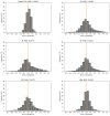
Fig 12. Model1.2D performs better than all human experts.

Histograms of error as difference between prediction and true value, and MSE (plot label) for the GNN (top left) and all experts for simulated 2D colonies from data set A (Table 1). The dashed orange line indicates zero error.

Fig 13. Model1.3D exhibits a low MSE.

Histogram of error as difference between prediction and true value, and MSE (plot label) for the GNN trained and tested on data set B (Table 1). The dashed orange line indicates zero error.

Fig 14. in vitro organoids are predicted to have rather low dispersion parameter.

Dispersion parameter values predicted by Model 1.3D for 24 h (left) and 48 h (right) organoids.

Fig 15. Schematic overview of the pattern reconstruction approach.

The color of the cells indicates their cell fates. Highlighted cells are used as input for the machine learning algorithm which outputs a prediction for the grey cell.

Fig 16. Model2.2D performs best for seven neighbors.

Overview of the testing accuracy of Model2.2D predicting simulated 2D colonies with q=0.1 dependent on the number of neighbors taken as an input for the model. Please note that for a clearer display, the y-axis starts at 65%.

Fig 17. Low and high values of q show best predictability with Model2.2D.

Overview of the predictability of simulated 2D colonies with different dispersion parameters q. All trainings and predictions were made under the same conditions with Model2.2D. The greyscale color gradient indicates the predictability of the different data, based on the accuracy.

Fig 18. Model2.3D for simulated 3D organoids performs best for 12–15 neighbors.

Overview of the accuracy of Model2.3D predicting simulated 3D organoids with q=0.1 dependent on the number of neighbors taken as an input for the model. Please note that for a clearer display, the y-axis starts at 65%.

Fig 19. Model 2.2D and 2.3D outperform human expert predictions.

Accuracy of Model2.2 on different simulated 2D colony and organoid data in comparison with humans. Both, Model2.2D and Human were tested with seven neighbors, using two-dimensional simulated colony data (data set C, Table 1). Model2.3D was run with 14 neighbors on three-dimensional simulated organoid data (data set D, Table 1). Please note that for a clearer display, the y-axis starts at 40%.

Fig 20. Model 2.3D trained on data set D (Table 1) performs better for high qs.

Accuracy of Model2.3D for different values of q. As training data, we used the complete data set D (Table 1) without splitting it according to the value of q. Please note that for a clearer display, the y-axis starts at 65%.

Fig 21. Model3 for ICM organoids performs best for 8–12 neighbors.

Overview of the accuracy of Model3 predicting ICM organoid data dependent on the number of neighbors taken as an input for the model. Please note that for a clearer display, the y-axis starts at 65%.

Fig 22. Confusion Matrix of cells pooled from six ICM organoids for Model2.3D.

All predictions were plotted against all labels, shown as percentages and totals in the confusion matrix (left). Confusion matrix in which the row entries were normalized to 1 (right). Test predictions made with the fully trained Model3 on cells from six different ICM organoids.

References

1. Kang M, Piliszek A, Artus J, Hadjantonakis AK. FGF4 is required for lineage restriction and salt-and-pepper distribution of primitive endoderm factors but not their initial expression in the mouse. Development. 2013;140(2):267–279. doi: 10.1242/dev.084996 - DOI - PMC - PubMed
1. Fischer SC, Corujo-Simon E, Lilao-Garzon J, Stelzer EHK, Muñoz-Descalzo S. The transition from local to global patterns governs the differentiation of mouse blastocysts. PLOS ONE. 2020;15:e0233030. doi: 10.1371/journal.pone.0233030 - DOI - PMC - PubMed
1. Schröter C, Rué P, Mackenzie JP, Arias AM. FGF/MAPK signaling sets the switching threshold of a bistable circuit controlling cell fate decisions in embryonic stem cells. Development. 2015;142(24):4205–4216. doi: 10.1242/dev.127530 - DOI - PMC - PubMed
1. Rivron NC, Frias-Aldeguer J, Vrij EJ, Boisset JC, Korving J, Vivié J, et al.. Blastocyst-like structures generated solely from stem cells. Nature. 2018;557(7703):106. doi: 10.1038/s41586-018-0051-0 - DOI - PubMed
1. Mathew B, Muñoz-Descalzo S, Corujo-Simon E, Schröter C, Stelzer EHK, Fischer SC. Mouse ICM Organoids Reveal Three-Dimensional Cell Fate Clustering. Biophysical Journal. 2019;116:127–141. doi: 10.1016/j.bpj.2018.11.011 - DOI - PMC - PubMed