Transferring principles of solid-state and Laplace NMR to the field of in vivo brain MRI

Abstract

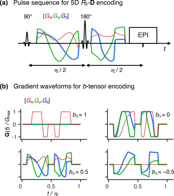
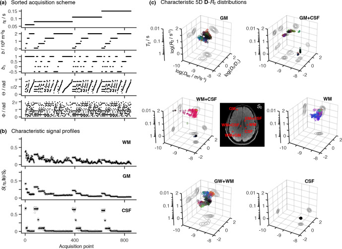
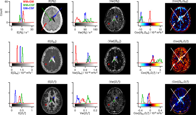
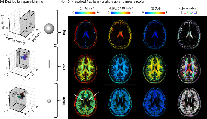
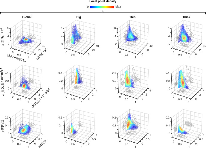
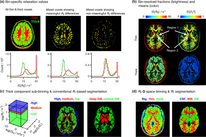
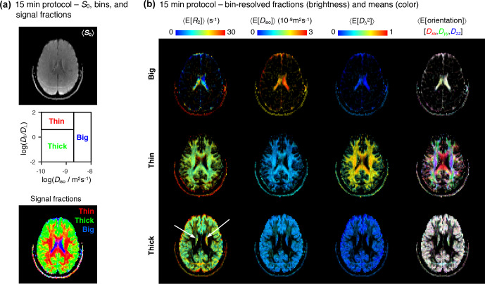
Magnetic resonance imaging (MRI) is the primary method for noninvasive investigations of the human brain in health, disease, and development but yields data that are difficult to interpret whenever the millimeter-scale voxels contain multiple microscopic tissue environments with different chemical and structural properties. We propose a novel MRI framework to quantify the microscopic heterogeneity of the living human brain as spatially resolved five-dimensional relaxation-diffusion distributions by augmenting a conventional diffusion-weighted imaging sequence with signal encoding principles from multidimensional solid-state nuclear magnetic resonance (NMR) spectroscopy, relaxation-diffusion correlation methods from Laplace NMR of porous media, and Monte Carlo data inversion. The high dimensionality of the distribution space allows resolution of multiple microscopic environments within each heterogeneous voxel as well as their individual characterization with novel statistical measures that combine the chemical sensitivity of the relaxation rates with the link between microstructure and the anisotropic diffusivity of tissue water. The proposed framework is demonstrated on a healthy volunteer using both exhaustive and clinically viable acquisition protocols.

Figure 1

Acquisition protocol for 5D relaxation–diffusion MRI. (a) Pulse sequence for acquiring images encoded for relaxation and diffusion in a 5D space defined by the echo time ${\mathit{\tau }}_{\mathrm{E}}$ , and $b$ -tensor trace $b$ , normalized anisotropy $b_{\mathrm{\Delta }}$ , and orientation ( $\mathrm{\Theta }$ , $\mathrm{\Phi }$ ). An EPI image readout block acquires the spin echo produced by slice-selective 90 and 180 ${}^{\circ }$ radio-frequency pulses. The 180 ${}^{\circ }$ pulse is encased by a pair of gradient waveforms allowing for diffusion encoding according to principles from multidimensional solid-state NMR (Topgaard, 2017) (red, green, and blue lines). The signal is encoded for the transverse relaxation rate $R_{\mathrm{2}}$ by varying the value of ${\mathit{\tau }}_{\mathrm{E}}$ . (b) Numerically optimized gradient waveforms (Sjölund et al., 2015) yielding four distinct $b$ -tensor shapes ( $b_{\mathrm{\Delta }}=-\mathrm{0.5}$ , 0.0, 0.5, and 1) (Eriksson et al., 2015).

Figure 2

Representative 5D relaxation–diffusion encoded signals $S({\mathit{\tau }}_{\mathrm{E}},\mathbf{b})$ and distributions $P(R_{\mathrm{2}},\mathbf{D})$ for selected voxels in a living human brain. (a) Acquisition scheme showing ${\mathit{\tau }}_{\mathrm{E}}$ , $b$ , $b_{\mathrm{\Delta }}$ , $\mathrm{\Theta }$ , and $\mathrm{\Phi }$ as a function of acquisition point. (b) Experimental (gray circles) and fitted (black points) $S({\mathit{\tau }}_{\mathrm{E}},\mathbf{b})$ signals from three representative voxels containing white matter (WM), gray matter (GM), and cerebrospinal fluid (CSF). The presented signal data were acquired according to the scheme shown in panel (a) and is drawn with the same horizontal axis. (c) Nonparametric $R_{\mathrm{2}}$ - $\mathbf{D}$ distributions obtained for both pure (WM, GM, CSF) and mixed (WM $+$ GM, WM $+$ CSF, GM $+$ CSF) voxels. The discrete distributions are reported as scatter plots in a 3D space of the logarithms of the transverse relaxation rate $R_{\mathrm{2}}$ , isotropic diffusivity $D_{\mathrm{iso}}$ , and axial–radial diffusivity ratio $D_{\mathrm{|}\mathrm{|}}/D_{\perp }$ . An auxiliary relaxation time $T_{\mathrm{2}}$ scale was included along the $\log \left(R_{\mathrm{2}}\right)$ axis to aid the inspection of the $P(R_{\mathrm{2}},\mathbf{D})$ plots. The diffusion tensor orientation ( $\mathit{\theta }$ , $\mathit{\phi }$ ) is color-coded as [R,G,B]  $=[\cos \mathit{\phi }\sin \mathit{\theta },\sin \mathit{\phi }\sin \mathit{\theta },\cos \mathit{\theta }]\cdot |D_{\mathrm{|}\mathrm{|}}-D_{\perp }|/max(D_{\mathrm{|}\mathrm{|}},D_{\perp })$ , and the circle area is proportional to the statistical weight of the corresponding component. The contour lines on the sides of the plots represent projections of the 5D $P(R_{\mathrm{2}},\mathbf{D})$ distribution onto the respective 2D planes. Panels (b) and (c) display the signals $S({\mathit{\tau }}_{\mathrm{E}},\mathbf{b})$ and corresponding $P(R_{\mathrm{2}},\mathbf{D}$ ), respectively, for the same WM, GM, and CSF voxels.

Figure 3

Statistical measures derived from the relaxation–diffusion distributions. The ensemble of 96 distinct $P(R_{\mathrm{2}},\mathbf{D})$ solutions was used to calculate means E[ $x$ ], variances Var[ $x$ ], and covariances Cov[ $x$ , $y$ ] of all combinations of transverse relaxation rate $R_{\mathrm{2}}$ , isotropic diffusivity $D_{\mathrm{iso}}$ , and squared anisotropy ${D_{\mathrm{\Delta }}}^{\mathrm{2}}$ . The statistical measures were all derived from the entire $R_{\mathrm{2}}$ - $\mathbf{D}$ distribution space on a voxel-by-voxel basis. Histograms are used to represent the parameter sets calculated for three voxels containing binary mixtures of white matter (WM), gray matter (GM), and cerebrospinal fluid (CSF). Each histogram comprises 96 estimates of a single statistical measure. The averages of statistical measures, $\langle \mathrm{E}\left[x\right]\rangle$ , $\langle \mathrm{Var}\left[x\right]\rangle$ and $\langle \mathrm{Cov}[x,y]\rangle$ , are displayed as parameter maps whose color scales are given by the bars along the abscissas of the histograms. The crosses and arrows identify the heterogeneous voxels analyzed in the histograms; notice that the signaled points correspond to the average (as measured by the median) of the ensembles of plausible solutions shown in the histograms.

Figure 4

Parameter maps with bin-resolved means of the relaxation–diffusion distributions. (a) Division of the $R_{\mathrm{2}}$ - $\mathbf{D}$ distribution space into different bins. The distribution space was separated into three bins (gray volumes) named “big”, “thin”, and “thick” that loosely capture the diffusion features of cerebrospinal fluid CSF, white matter WM, and gray matter GM, respectively. The 3D scatter plots display the nonparametric $R_{\mathrm{2}}$ - $\mathbf{D}$ distributions corresponding to the CSF (top), WM (middle), and GM (bottom) voxels selected in Fig. 2. Superquadric tensor glyphs are used to illustrate the representative $\mathbf{D}$ captured by each bin. (b) Parameter maps of average per-bin means (color) of transverse relaxation rate $\langle \mathrm{E}\left[R_{\mathrm{2}}\right]\rangle$ , isotropic diffusivity $\langle \mathrm{E}\left[D_{\mathrm{iso}}\right]\rangle$ , squared anisotropy $\langle \mathrm{E}\left[{D_{\mathrm{\Delta }}}^{\mathrm{2}}\right]\rangle$ , and diffusion tensor orientation $\langle \mathrm{E}$ [Orientation] $\rangle$ . The orientation maps (column 4) are color-coded as [R,G,B]  $=[D_{xx},D_{yy},D_{zz}]/max(D_{xx},D_{yy},D_{zz})$ , where $D_{ii}$ are the diagonal elements of laboratory-framed average diffusion tensors estimated from the various distribution bins. Brightness indicates the signal fractions corresponding to the big (row 1), thin (row 2), and thick (row 3) bins. The white arrows identify deep gray-matter structures.

Figure 5

Uncertainty estimation of the statistical measures derived from the relaxation–diffusion distributions. 3D density (color) scatter plots show the relationship between average initial signal intensity $\langle S_{\mathrm{0}}\rangle$ , the average of mean values derived from the $R_{\mathrm{2}}$ - $\mathbf{D}$ distributions $\langle \mathrm{E}\left[x\right]\rangle$ , and their corresponding uncertainties $\mathit{\sigma }\left[\mathrm{E}\right[x\left]\right]$ . For display purposes, signal intensity values were normalized to the maximum recorded $\langle S_{\mathrm{0}}\rangle$ , $max(\langle S_{\mathrm{0}}\rangle )$ . The contour lines on the side planes show 2D projections of the point density function defining the distribution of data points. The average mean values of transverse relaxation rate $\langle \mathrm{E}\left[R_{\mathrm{2}}\right]\rangle$ (row 1), isotropic diffusivity $\langle \mathrm{E}\left[D_{\mathrm{iso}}\right]\rangle$ (row 2), and squared anisotropy $\langle \mathrm{E}\left[{D_{\mathrm{\Delta }}}^{\mathrm{2}}\right]\rangle$ (row 3) were computed from all voxels whose $\langle S_{\mathrm{0}}\rangle$ was greater than 5 % of $max(\langle S_{\mathrm{0}}\rangle )$ . The resulting dataset comprises 55 327 voxels spread throughout all slices of the acquired 3D volume. The uncertainties of $\langle \mathrm{E}\left[R_{\mathrm{2}}\right]\rangle$ , $\langle \mathrm{E}\left[D_{\mathrm{iso}}\right]\rangle$ , and $\langle \mathrm{E}\left[{D_{\mathrm{\Delta }}}^{\mathrm{2}}\right]\rangle$ correspond to the median absolute deviation between measures extracted from 96 independent solutions of Equation (2): $\mathit{\sigma }\left[\mathrm{E}\right[R_{\mathrm{2}}\left]\right]$ , $\mathit{\sigma }\left[\mathrm{E}\right[D_{\mathrm{iso}}\left]\right)$ , and $\mathit{\sigma }\left[\mathrm{E}\right[{D_{\mathrm{\Delta }}}^{\mathrm{2}}\left]\right]$ , respectively. All displayed data were derived from both the entire $R_{\mathrm{2}}$ - $\mathbf{D}$ space (column 1), and the “big” (column 2), “thin” (column 3), and “thick” (column 4) bins defined in Fig. 4a.

Figure 6

Per-bin relaxation properties and tissue composition. (a) Transverse relaxation properties specific to each of the “thin” (red) and “thick” (green) bins defined in Fig. 4a. The color-coded composite images (top) and histograms (bottom) display the fractional populations and average mean transverse relaxation values $\langle \mathrm{E}\left[R_{\mathrm{2}}\right]\rangle$ of the two bins. The first column displays all of the thin and thick voxels, while the two other columns focus on thin $+$ thick mixtures wherein the bin-specific $\langle \mathrm{E}\left[R_{\mathrm{2}}\right]\rangle$ values exhibit either significant (second column) or nonsignificant (third column) differences. (b) Bin-resolved signal fractions (brightness) and average per-bin means (color) of $R_{\mathrm{2}}$ , and squared anisotropy ${D_{\mathrm{\Delta }}}^{\mathrm{2}}$ . Regions 1 and 2 identify microstructural properties singled-out in the Results section. (c) Subdivision of the thick bin into three different $R_{\mathrm{2}}$ subspaces. The contributions from different sub-bins are compared with a high-resolution $R_{\mathrm{1}}$ -weighted image segmented into four different tissues: white matter WM, cortical gray matter (GM), deep GM, and cerebrospinal fluid (CSF). Additive color maps display the spatial distribution of sub-bin fractions (from low to high $R_{\mathrm{2}}$ : green, red, blue), and of cortical (green) and deep (red) GM. (d) Color-coded composite images showing the contributions of different bins (red  $=$  thin, green  $=$  thick, blue  $=$  big) and conventional $R_{\mathrm{1}}$ -based segmentation labels (red  $=$  WM, green  $=$  cortical  $+$  deep GM, blue  $=$  CSF).

Figure 7

15 min protocol – bin-resolved signal contributions and mean parameter maps. (a) Map of average initial signal intensity $\langle S_{\mathrm{0}}\rangle$ (top); subdivision of the diffusion space into the “big”, “thin”, and “thick” bins (middle); color-coded composite map of per-bin signal contributions (bottom). The colors in the bottom identify the fractions from different bins: [R,G,B]  $=$ [thin,thick,big]. (b) Parameter maps of average per-bin means (color) of transverse relaxation rate $\langle \mathrm{E}\left[R_{\mathrm{2}}\right]\rangle$ , isotropic diffusivity $\langle \mathrm{E}\left[D_{\mathrm{iso}}\right]\rangle$ , squared anisotropy $\langle \mathrm{E}\left[{D_{\mathrm{\Delta }}}^{\mathrm{2}}\right]\rangle$ , and diffusion tensor orientation $\langle \mathrm{E}$ [Orientation] $\rangle$ . The color and brightness of the various maps follows the same convention as Fig. 4b.

References

1. Assaf Y. Imaging laminar structures in the gray matter with diffusion MRI. Neuroimage. 2018;197:677–688. doi: 10.1016/j.neuroimage.2017.12.096. - DOI - PubMed
1. Bak M, Nielsen NC. REPULSION, a novel approach to efficient powder averaging in solid-state NMR. J Magn Reson. 1997;125:132–139. doi: 10.1006/jmre.1996.1087. - DOI - PubMed
1. Barth M, Breuer F, Koopmans PJ, Norris DG, Poser BA. Simultaneous multislice (SMS) imaging techniques. Magn Reson Med. 2016;75:63–81. doi: 10.1002/mrm.25897. - DOI - PMC - PubMed
1. Basser PJ, Pierpaoli C. Microstructural and physiological features of tissues elucidated by quantitative-diffusion-tensor MRI. J Magn Reson Ser B. 1996;111:209–219. doi: 10.1016/j.jmr.2011.09.022. - DOI - PubMed
1. Bazin P-L, Alkemade A, van der Zwaag W, Caan M, Mulder M, Forstmann BU. Denoising High-Field Multi-Dimensional MRI With Local Complex PCA. Front Neurosci-Switz. 2019;13:1066. doi: 10.3389/fnins.2019.01066. - DOI - PMC - PubMed
LinkOut - more resources