Effects of stochastic coding on olfactory discrimination in flies and mice

Abstract

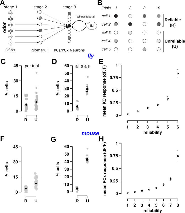
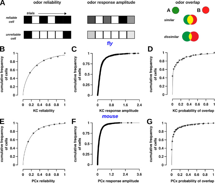
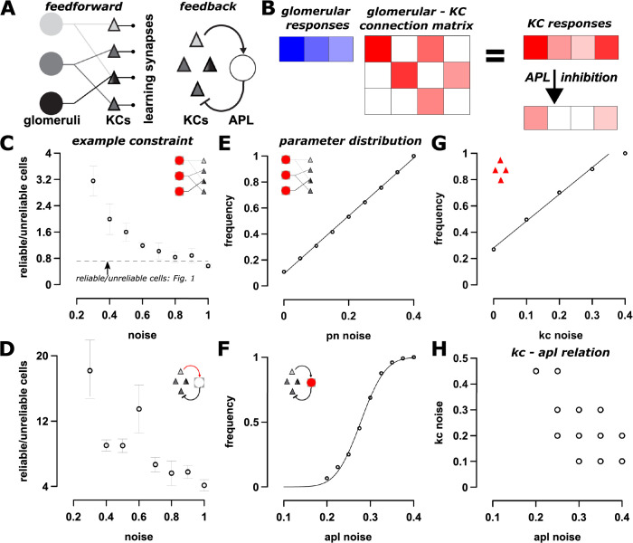
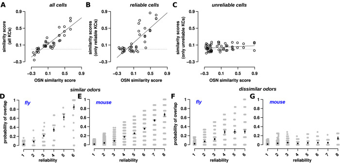
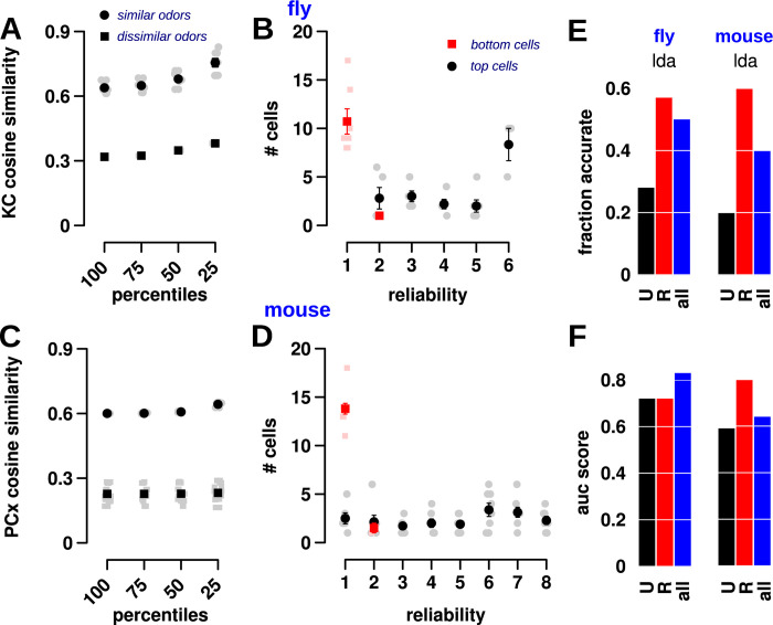
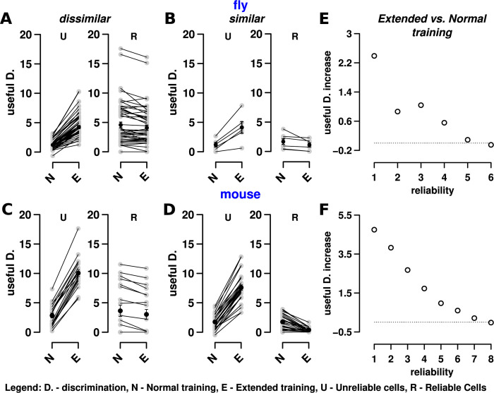
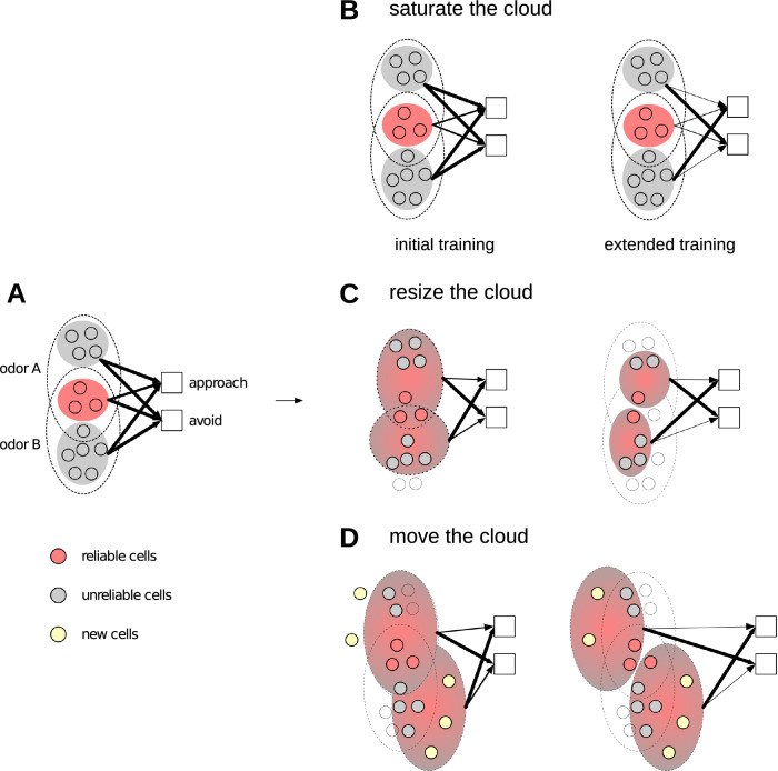
Sparse coding can improve discrimination of sensory stimuli by reducing overlap between their representations. Two factors, however, can offset sparse coding's benefits: similar sensory stimuli have significant overlap and responses vary across trials. To elucidate the effects of these 2 factors, we analyzed odor responses in the fly and mouse olfactory regions implicated in learning and discrimination-the mushroom body (MB) and the piriform cortex (PCx). We found that neuronal responses fall along a continuum from extremely reliable across trials to extremely variable or stochastic. Computationally, we show that the observed variability arises from noise within central circuits rather than sensory noise. We propose this coding scheme to be advantageous for coarse- and fine-odor discrimination. More reliable cells enable quick discrimination between dissimilar odors. For similar odors, however, these cells overlap and do not provide distinguishing information. By contrast, more unreliable cells are decorrelated for similar odors, providing distinguishing information, though these benefits only accrue with extended training with more trials. Overall, we have uncovered a conserved, stochastic coding scheme in vertebrates and invertebrates, and we identify a candidate mechanism, based on variability in a winner-take-all (WTA) inhibitory circuit, that improves discrimination with training.

Fig 1. Response reliability is similar in third-order neurons of the fly and mouse olfactory circuit.

(A) Schematic of the first 3 stages of fly and mouse olfactory circuits. In stage 1, odors are sensed by OSNs. In stage 2, OSNs pass odor information onto glomeruli structures in the antenna lobe (flies) or olfactory bulb (mice). In stage 3, odor information is passed to a larger number of KCs in the MB (flies) or cells in the PCx (mouse). Stage 3 cells are sparsified by an inhibitory WTA circuit, which suppresses the activity of less responsive cells. (B) An example schematic showing response variability in stage 3 cells. Some cells (cells 1 and 2) have a large response in most trials (indicated by R for reliable cells), while most cells respond in ≤ half the trials with a smaller response (indicated by U for unreliable cells). (C–E) Responses of 124 KCs in flies for 7 odors with 6 trials per odor; data from [9]. (C) The percentage of responsive KCs that are reliable (5.26 ± 0.7%) and unreliable (7.23 ± 0.84%) per odor trial. There are 42 gray points, 1 per odor-trial pair. (D) The percentage of KCs that are reliable (6.1 ± 1.9%) and unreliable (29.0 ± 3.16%) across all trials. Each gray point is an odor and the black point represents the mean. There are many more unreliable cells than reliable cells. (E) The mean response of a KC (y-axis) increases with the cell’s reliability (x-axis). The measure of the fit, using linear regression on a log-plot, is shown in panel A in Fig A in S1 Text (r = 0.97). (F–H) Responses of 285 PCx cells in mice for 10 odors with 8 trials per odor; data collected in this study. (F) The percentage of responsive PCx cells that are reliable (3.3 ± 0.2%) and unreliable (8.7 ± 0.4%) per trial. There are 80 gray points, 1 per odor-trial pair. (G) The percentage of PCx cells that are reliable (4.4 ± 0.7%) and unreliable (43.1 ± 1.8%) across all trials. Again, there are many more unreliable cells than reliable cells. (H) The mean response of a PCx cell (y-axis) increases with the cell’s reliability (x-axis). The measure of the fit is shown in panel B in Fig A in S1 Text (r = 0.98). Error bars in all panels indicate mean ± SEM. Datasets used in these plots for flies (A–E) and mice (F–H) are stored within the Zenodo and Dandi repositories as the fly main dataset and dataset 164, respectively. Links on accessing the data are in the Data Availability section, and the data repositories contain further details on the datasets. The data underlying the graphs shown in the figure can be found in S1 Data. KC, Kenyon cell; MB, mushroom body; OSN, olfactory sensory neuron; PCx, piriform cortex; SEM, standard error of the mean; WTA, winner-take-all.

Fig 2. Cell reliability, response size, and odor specificity follow a continuous distribution.

(A) Schematic of 3 response properties that were examined for odors and odor-pairs. Odor reliability refers to the number of trials for which a cell is responsive. Each trial is depicted by a grid square, and black color indicates a response. Cells that respond in more than half the trials were classified as reliable; all other responsive cells were unreliable. Odor response size is the firing rate of the cell in individual trials, as measured by Ca²⁺ fluorescence. The top line shows a cell with a large response, where the intensity of gray denotes size of response. Odor overlap is the probability that the cell will respond to both odors. The odor overlap here is shown in yellow and decreases for dissimilar odors (bottom) compared to similar odors (top). (B, E) Cumulative frequency histograms showing the distribution of reliabilities for KCs (flies) and PCx cells (mice). Each circle represents the cumulative probability for cells with a reliability value represented on the x-axis. The points are fit by Gamma distributions with shape = 0.64, scale = 0.42 (for B, fly) and shape = 0.64, scale = 0.17 (for E, mice). The significance of the Gamma distribution is that it is a maximum entropy code and optimizes for the most stimuli that can be encoded (see text). (C, F) Cumulative frequency histograms for response sizes in both flies and mice are well fit by Gamma distributions with shape = 0.77, scale = 0.28 (for C, fly) and shape = 0.70, scale = 0.24 (for F, mice). (D, G) Cumulative frequency histograms for the overlap of cells between odor-pairs in both flies and mice, also fit using Gamma distributions with shape = 0.19, scale = 0.60 (for D, fly) and shape = 0.18, scale = 0.35 (for G, mice). Datasets used in these plots for flies (B–D) and mice (E–G) are stored within the Zenodo and Dandi repositories as the main dataset for flies and dataset 164 for mice, respectively. The data underlying the graphs shown in the figure can be found in S2 Data. KC, Kenyon cell; PCx, piriform cortex.

Fig 3. A WTA mechanism is needed for generating stochastic codes.

(A, left) Schematic of information transfer in the fly olfactory circuit. Odor information from OSNs is passed from glomeruli to KCs (via PNs) in the MB. KCs synapse with MBONs that influence behavior. The KC→MBON synapses are subject to synaptic plasticity. (A, right) The WTA circuit in MB, where all KCs activate the inhibitory APL neuron that in turn feeds back and inhibits all KCs. (B) A schematic of the linear rate firing model. The PN response to odors is depicted in blue, and their connection matrix with KCs is denoted in red. With a linear rate firing model, we take a product of the odor vector and connection matrix to get the KC response, which is sparsified by the APL neuron inhibitory feedback. (C, D) Examples of how the model was checked against constraints. Model simulations show that injecting noise in (C) PNs or (D) KC-APL synapses produces different ratios of reliable to unreliable cells responding per trial. The straight line in the plots denotes a reliable/unreliable cell ratio of 0.72 observed with experimental MB responses (Fig 1). For both plots, the x-axis denotes the fraction of injected noise. Thus, 1 denotes that noise levels are 100% of signal. (E–G) Distribution of individual parameters that make up the “successful” parameter sets. Here, the 6 parameters were varied over a large range (Methods), and we have plotted individual cumulative distributions to show the dependence of the stochastic code on various parameters. (E) PN noise is uniformly distributed. (F) APL noise is normally distributed with a mean of 0.28. (G) KC noise cumulative distribution, where the initial noise is uniformly distributed. (H) There is a an inverse relationship between APL and KC noise. With increasing KC noise, the amount of APL noise that is required for the stochastic code is reduced. Error bars indicate SEM. See Table B in S1 Text, Fig J in S1 Text, Fig K in S1 Text, Fig G in S1 Text, and Methods for more details. APL, anterior paired lateral; KC, Kenyon cell; MB, mushroom body; MBON, MB output neuron; OSN, olfactory sensory neuron; PN, projection neuron; WTA, winner-take-all.

Fig 4. Reliable and unreliable cells differ in their response to odors.

(A) The similarity between odor pairs was calculated based on OSN response correlation in the fly’s antenna [68] (x-axis) and KC response correlation in the fly’s MB (y-axis). Each circle denotes 1 odor-pair. Similarity between odor pairs was calculated via Pearson’s correlation of response vectors. When considering all KCs, odor similarity was highly correlated (r = 0.89). The equation for the line fit is y = 0.78x. The dotted line (y = 0) in this plot and in B and C indicates the value at which there is no correlation. (B) When considering only reliable KCs, odor similarity is also highly correlated (r = 0.80). The equation for the line fit is y = 0.88x. (C) In contrast, the similarity between odor-pair responses for only unreliable cells has very low correlation (r = 0.20). The line fit has equation y = 0.05x, i.e., the slope is close to 0. In other words, odor pairs that are dissimilar (left part of the x-axis) have only slightly less correlation than similar odor pairs (right part of the x-axis). (D, E) In both flies and mice, reliable cells overlap more than unreliable cells for similar odors (i.e., odor-pairs with correlation > 0.5 in their odor responses). Here, overlap is the probability that a cell will respond to both odors, e.g., if the probability of response to the 2 odors is 1/6 and 3/6, the overlap is 3/36 or 1/12. Each gray circle shows the overlap between 2 odors for a single cell, whose reliability for the first of the odor pair is shown on the y-axis. Pearson’s correlation between overlap and reliability is 0.87 and 0.91, for flies and mouse, respectively. (F, G) For dissimilar odors (correlation < 0.15), while reliable cells have a higher overlap than unreliable cells, the increase in overlap is much less than for similar odors shown in (D, E). Correlation is 0.55 and 0.33 for linear fits, with slopes of 0.05 and 0.009, respectively, for flies and mice. Error bars indicate SEM. Datasets used in these plots for flies (A–C, D, F) and mice (E, G) are stored within the Zenodo and Dandi repositories as the fly main dataset and dataset 164, respectively (see Data Availability section). Additionally plots A–C used the following supplementary fly datasets: 09042009, 110108, 110109_1, 110109_2. The data underlying the graphs shown in the figure can be found in S3 Data. KC, Kenyon cell; MB, mushroom body; OSN, olfactory sensory neuron.

Fig 5. Reliable and unreliable cells contribute differently to odor discrimination.

(A) The cosine similarity (y-axis) for the top 25, 50, 75, and 100% of responsive KCs (x-axis) for similar odors (correlation > 0.5, top circles) and dissimilar odors (correlation ≤ 0.15, bottom squares). Each square and circle represent odor pairs. The top 25% most responsive cells are more similar than the responses of cells in other percentiles. In other words, the top 25% most responsive cells have the highest overlap for similar odors, and thus they provide less discriminatory power, compared to cells in other percentiles. Cells with high responses demonstrate the lowest overlap for dissimilar odors, but the highest overlap for similar odors. Sparse coding methods typically retain only the highest responding neurons (here, the top 25% of cells). Thus, these results challenge whether sparse coding alone is sufficient for discriminating similar odors. (B) The number of cells at each reliability level for the top 25% (black circle) and bottom 25% (red square) of cells. Most of the top 25% of cells are reliable, while nearly all of the bottom 25% of cells have the lowest reliability. (C) The same plot for mice as (A), showing similar trends. (D) The same plot for mice as (B), showing similar trends. (E) Simple machine learning algorithms (LDA) applied to reliable, unreliable, and all cells show that reliable cells are significantly better at classification than unreliable cells. Compare the length of the red bars (reliable, R) to the black bars (unreliable, UR), where the length of the bar denotes the fraction of correct classifications. The performance of the decoder with all cells (blue bars) is similar to reliable cells, though slightly less. See Methods and Table C in S1 Text for algorithm details and parameters for the LDA decoder and the training and test sets. See panels G and H in Fig C in S1 Text for analogous results with SVM and kNN decoders. (F) AUC (averaged over all pairs of odors) for assessing the pair-wise discrimination performance of unreliable (U, black bars), reliable (R, red bars), and all (blue bars) cells for LDA. Reliable cells, on average, have slightly higher AUC measures. Unlike accuracy measures from (D); however, unreliable cells (in black) show significantly higher AUC, suggesting that they provide significant information for distinguishing odors. See panel D in Fig C in S1 Text for area under the ROC (AUC) measure for assessing performance of the classifiers specifically for similar and dissimilar odors. Datasets used in these plots for flies (A, B, E) and mice (C, D, F) are stored within the Zenodo and Dandi repositories as the fly main dataset and mouse dataset 164, respectively. The data underlying the graphs shown in the figure can be found in S4 Data. AUC, area under the curve; KC, Kenyon cell; kNN, k nearest neighbor; LDA, linear discriminant analysis; SVM, support vector machine.

Fig 6. Unreliable cells contribute more to discrimination of similar odors.

Extended learning increases the amount of discriminatory power between odor-pairs. Odor-pairs are split into dissimilar (A, C) odor-pairs, whose correlation coefficient is ≤<0.15, and similar (B, D) odor-pairs with a correlation > 0.5. (A) Shown are 2 plots of how extended (E, x-axis) and normal (N, x-axis) training affect the contributions of (y-axis) unreliable cells (left plot, UR) and reliable cells (right plot, R) towards discrimination (termed useful Discrimination) of dissimilar odors. Each gray point represents the discrimination measure (Eq 2) for an odor-pair. Discrimination calculations for the fly are based on data from [9]. Unreliable cell contributions increase with extended training, to match the contributions of reliable cells. (B) Similar plots as (A) for similar odors. Here, too, extended training increases the discrimination contribution of unreliable (UR) cells. For reliable cells, however, contributions are maintained or reduced; (C, D) are equivalent calculations for the mouse dataset shown in Fig 1. (E, F) The improvement in discrimination from normal to extended training for similar odor-pairs in flies (E) and mice (F). Each circle represents the contribution of cells in a reliability class (x-axis) towards the ability to discriminate similar odors with extended training compared to normal training (y-axis). The highest contribution towards discrimination comes from cells with a reliability of 1, and the contributions decrease as the reliability increases. The dotted lines (y = 0) indicate the value at which there is no change in useful discrimination. Datasets used in these plots for flies (A, B, E) and mice (C, D, F) are stored within the Zenodo and Dandi repositories as the fly main dataset and mouse dataset 164 (links in Data Availability section). Additionally, plots A–C used the following supplementary fly datasets: 09042009, 110106_4, 110107_2, 110109_1, and 110109_2. The data underlying the graphs shown in the figure can be found in S5 Data.

Fig 7. Three possible models of fine-discrimination.

(A) The stimulus representations in the untrained animal. For each odor, the dotted ovals enclose the cells that respond to the odor (unreliable cells are gray, reliable cells are pink). The unreliable cells are mostly non-overlapping for the 2 odors, whereas the reliable cells overlap exactly. The thickness of the arrows denotes the total strength from the 3 sets of cells to the 2 downstream neurons that drive approach or avoidance behavior. Initially, all arrows are of the same strength. (B) Saturating the cloud. With initial training (left), the strength of downstream synapses of reliable cells saturates (i.e., weakens to near zero), but synapses of unreliable cells barely change their strength. Consequently, as reliable cell overlap is high between the 2 odors, approach/avoid neurons receive equal input, and the animal is unable to discriminate. With extended training (right), the downstream synapses of unreliable cells also saturate, driving the 2 stimuli apart, as depicted by the thicker arrows. The connection strengths to the approach MBON are much weaker than to the avoid MBON, and therefore odor A and B are distinguishable. (C) Resize the cloud. The stimulus representation shrinks to only include cells that are non-overlapping between the 2 stimuli (e.g., the shared reliable cells are turned off). While some resizing may occur with normal training, with extended training, the 2 stimuli are further driven apart, enabling the animal to discriminate the 2 odors. (D) Move the cloud. Some mechanism (most likely driven by unreliable cells, the cells that are most unlike between similar odors) rearranges the stimulus ensemble response to include new cells, or converts unreliable to reliable cells that do not overlap, and thus improve discrimination. MBON, MB output neuron.

Fig 8. Detecting signals with calcium imaging.

(A–E) Mouse calcium imaging data registration and segmentation. (A) Top: Maximum projection GRIN lens FOV of the T-series for each plane imaged. Bar: 100 μm. Bottom: Corresponding ROIs segmented. (B) Pixel shift in the x-axis (left) and y-axis (right) during registration at each represented by frames on the x-axis. (C) Size (in pixels) distribution of each of the segmented ROIs. (D) Peak of phase correlation between frame and reference image at each time point. (E) Magnitude of the shifts (both rigid and non-rigid) for each PC of the registered movie. (F–I) Fly calcium imaging analysis. (F) A few example traces of different significant cells. The dotted line is y = 0 and indicates the value at which Ca²⁺ activity is 0. (G) A cumulative distribution of the base (black) and signal (red) means. The signal follows a Gamma distribution as we showed in the paper (there is a little bit of a left skew), while the base mean is a very good fit for a Gaussian. The vertical dotted line (x = 0) denotes no response. (H, I) Plot of the base (left) and signal (right) means. There are 918 cells in all. The amount of overlap is about 90 cells for both responses, and 90 of the base means are above the lowest signal mean response. And, 90 of the signal means are below the highest base mean. We took the overlapping population of cells whose base means were above the lowest signal mean response, and re-plotted their and base and signals means while joining base and signal means for the same cells. We found that in these cells, all base means are lower than their signal means. Dotted line in (H) denotes the line (x = 0) denoting no response. See the Data Availability section for details on the 2 datasets used here: the fly main dataset (F–I) on Zenodo, and mouse dataset 164 (A–E) on Dandi. The data underlying the graphs shown in the figure can be found in S6 Data. FOV, field of view; PC, principal component; ROI, region of interest.

References

1. Field DJ. What Is the Goal of Sensory Coding? Neural Comput. 1994;6(4):559–601. doi: 10.1162/neco.1994.6.4.559 - DOI
1. Barth AL, Poulet JF. Experimental evidence for sparse firing in the neocortex. Trends Neurosci. 2012;35(6):345–355. doi: 10.1016/j.tins.2012.03.008 - DOI - PubMed
1. Lin AC, Bygrave AM, de Calignon A, Lee T, Miesenbøck G. Sparse, decorrelated odor coding in the mushroom body enhances learned odor discrimination. Nat Neurosci. 2014;17(4):559–568. doi: 10.1038/nn.3660 - DOI - PMC - PubMed
1. Attwell D, Laughlin SB. An energy budget for signaling in the grey matter of the brain. J Cereb Blood Flow Metab. 2001;21(10):1133–1145. doi: 10.1097/00004647-200110000-00001 - DOI - PubMed
1. Vinje WE, Gallant JL. Sparse coding and decorrelation in primary visual cortex during natural vision. Science. 2000;287(5456):1273–1276. doi: 10.1126/science.287.5456.1273 - DOI - PubMed