Bayesian traction force estimation using cell boundary-dependent force priors

Abstract

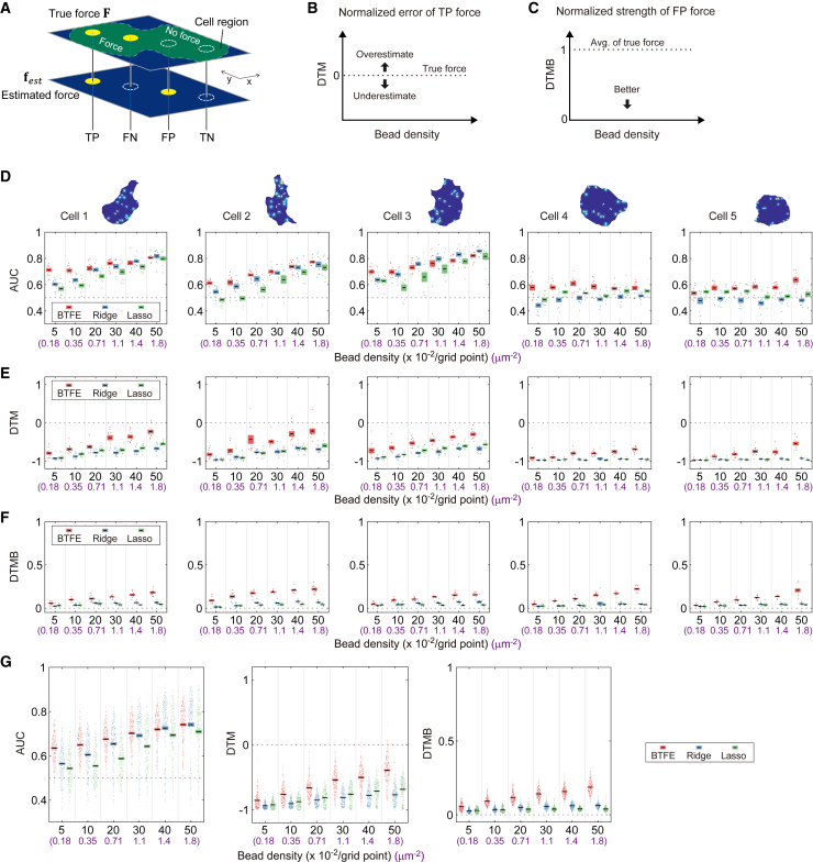
Understanding the principles of cell migration necessitates measurements of the forces generated by cells. In traction force microscopy (TFM), fluorescent beads are placed on a substrate's surface and the substrate strain caused by the cell traction force is observed as displacement of the beads. Mathematical analysis can estimate traction force from bead displacement. However, most algorithms estimate substrate stresses independently of cell boundary, which results in poor estimation accuracy in low-density bead environments. To achieve accurate force estimation at low density, we proposed a Bayesian traction force estimation (BTFE) algorithm that incorporates cell-boundary-dependent force as a prior. We evaluated the performance of the proposed algorithm using synthetic data generated with mathematical models of cells and TFM substrates. BTFE outperformed other methods, especially in low-density bead conditions. In addition, the BTFE algorithm provided a reasonable force estimation using TFM images from the experiment.

Figure 1

Diagram of Bayesian framework for estimating cell traction force using cell boundary priors. (A) Overview of traction force microscopy (TFM), a technique for measuring the force ($\mathbf{F}$; red arrows) exerted by a cell (green) on a substrate. In TFM, fluorescent beads on the surface of the substrate ($\mathbf{u}$; blue circles and arrows) move in response to the cell’s traction force, allowing the force to be calculated through inverse analysis of the bead displacement. (B) Main source of cellular force, which is generated by the polymerization of actin molecules at the cell edge, forming actin filaments that push against the membrane. The reaction force of this polymerization causes the retrograde flow of actin filaments (black arrow) in an intracellular direction. The mechanical linkage between the actin filaments and the substrate, mediated by adhesion and clutch molecules, allows the retrograde flow to produce a traction force (red arrow) (C) Force estimation with magnitude constraints (ridge regression) reduces the force magnitude to avoid overfitting to the observed bead displacement. (D) Force estimation by number constraint (lasso regression) explains the bead displacement with only a small number of forces. (E) Force-estimation method proposed in the present study incorporates a cell boundary constraint, assuming that forces limited to the cellular region induce displacement of extracellular beads. (F) Conceptual diagram of Bayesian force estimation is shown, in which a posterior distribution ($P\left(\mathbf{F}|\mathbf{u}\right)$; green) is obtained by satisfying the likelihood of the bead displacement u produced by the force $\mathit{F}$ ($P\left(\mathbf{u}|\mathit{F}\right)$; orange) and the prior distribution of the force that the cell is likely to generate on the basis of its boundary ($P\left(\mathbf{F}\right)$; yellow). The most plausible force is then estimated using MAP estimation.

Figure 2

Model of force prior derived from cell boundary. (A) A model of inward cellular traction force and its components. The prior probability distribution of the traction force at position $\mathbf{x}$, $P\left(\mathbf{f}\left(\mathbf{x}\right)\right)$, was defined as a 2D Gaussian distribution centered on the mean force ${\mathbf{f}}_{\mu }\left(x\right)$, which is divided into magnitude $m\left(\mathbf{x}\right)$ and direction $\mathbf{d}\left(\mathbf{x}\right)$. (B) Models for the magnitude $m\left(\mathbf{x}\right)$ and direction $\mathbf{d}\left(\mathbf{x}\right)$ functions. The magnitude function $m\left(\mathbf{x}\right)$ was set to be a nonnegative Gaussian function that depends on the distance $r\left(\mathbf{x}\right)$ from the nearest-neighbor edge. For the force direction function $\mathbf{d}\left(\mathbf{x}\right)$, the cell boundary was represented as a level-set function (LSF), and the unit vector of the gradient of the LSF was introduced. (C) Calculation of force magnitude and direction based on cell morphology. (a) Boundary of the cultured cell (solid line) compared to the boundary transformed using the LSF with MCF (see e). (b) Force magnitude $m\left(\mathbf{x}\right)$ calculated and visualized with a color gradient. (c) Cell boundary represented by the LSF $z=\varphi \left(\mathbf{x},0\right)$, with the gray region denoting the original cell boundary $\varphi \left(\mathbf{x},0\right)=0$. The z axis represents the distance from the cell edge: $-r\left(\mathbf{x}\right)$ for inside and $r\left(\mathbf{x}\right)$ for outside. (d) Gradient of the LSF inside the original cell boundary, with white arrows representing unit vectors. Regions with biologically inappropriate directions are indicated by the black arrow. (e) LSF after the cell has been transformed by time $\tau$ with MCF, $\varphi \left(\mathbf{x},\tau \right)$, where the time of the original cell boundary is zero. The gray region represents the interior of the transformed cell boundary $\varphi \left(\mathbf{x},\tau \right)=0$, with the edges represented by dotted circles in (a). (f) Gradient of the transformed boundary in (e), with white arrows indicating unit vectors of gradients inside the original cells, defined as $\mathbf{d}\left(\mathbf{x}\right)$.

Figure 3

Procedure for generating synthetic bead displacements and force estimation. (A) Workflow used to estimate traction forces from a synthetic dataset. First, we (a) extracted the model cell boundaries from cultured cells and (b) generated a virtual traction force inside it. The direction and magnitude of the forces are indicated by white arrows and the background color, respectively. Next, we (c) randomly distributed beads on the model substrate and (d) calculated their displacement due to traction force using the Boussinesq approximation ($\mathbf{u}=\mathrm{G}\mathbf{f}$). (e) The synthetic data for bead displacement were obtained by adding observation noise (2D Gaussian distribution with a standard deviation of 0.1 μm) to the displacement data. We used these noisy bead displacements to perform a Bayes estimation, ridge regression, and lasso traction force estimation and compared the estimated results to the correct cell forces to evaluate accuracy. (B) Cell models used for the synthetic dataset. We used five different cell boundaries and prepared different traction force distributions for each cell. For each cell boundary and traction force distribution pair, we prepared five different bead distributions.

Figure 4

Variation in force-estimation results with different bead densities and distributions. (A) Examples of introduced synthetic forces, with the force magnitude indicated by the background color. There are 20 individual force points, each with inwardly directed force. (B) Randomly scattered beads on the substrate model (density: 0.4 and 1.6 bead/μm²). The red lines indicate the bead displacements caused by the synthetic force shown in (A). Scale bar, 5 μm. (C–E) Comparison of estimation results from three different algorithms—(C) Bayes, (D) ridge, and (E) lasso—for a substrate model with a bead density of 0.4 bead/μm². All estimations were performed using the bead displacements shown in (B). (F–H) Same as (C)–(E) but with the substrate model having a bead density of 1.6 beads/μm². For all calculations, we placed estimated force points on a 30 × 30 grid.

Figure 5

Performance comparison of traction force-estimation algorithms. (A) A diagram showing force detection classifications and evaluation measures. Four types of force detection were used: true positive (TP), false negative (FN), false positive (FP), and true negative (TN), which were used to create an ROC curve for force detection accuracy. See Fig. S2 for details on how the area under the ROC curve (AUC) was calculated. Only forces estimated in the cellular region were targeted for any estimation algorithms. (B) Deviation of traction magnitude (DTM) is the ratio of the difference between the estimated TP force and the actual force magnitude. The closer to zero, the better. A value of −1 indicates that the estimated force is very close to zero. (C) Deviation of traction magnitude in the background (DTMB) indicates how large the estimated FP force was relative to the average magnitude of the actual force. The closer to zero, the better. (D) AUC versus bead density for the five cell boundaries (Fig. 3). Bead density is shown as the number of beads per grid point and the number of beads per unit area (purple). One force distribution was introduced in each cell boundary (top row), and evaluations were done for 10 different patterns of bead positions (bottom row). Cells 1–3 have relatively complex boundaries, whereas cells 4 and 5 are relatively round. (E) Same as (D) but for comparisons of DTM versus bead density. (F) Same as (D) but for comparisons of DTMB versus bead density. (G) The three evaluations for all data (n = 250; five different cell boundaries, five different force generation patterns, 10 different initial bead placements). The error bars in (D)–(G) represent the SE. For all calculations, we placed estimated force points on a 30 × 30 grid.

Figure 6

Comparison of force estimations using TFM images. (A) Images of neuronal growth-cone boundary and beads (top) and the corresponding Bayesian prior for force estimation (bottom). Cell boundary is represented by the white dashed line. (B) Bayesian force estimations using the beads in (A) (top) and focusing on pseudopods a, b, and c (bottom). The green arrow indicates cell migration direction. (C and D) Force estimation by ridge regression (C) and lasso regression (D) (top) and enlargements of the corresponding square areas to a, b, and c in (B) (bottom). Force estimation using ridge regression (C) and lasso regression (D) (top) with enlargements of corresponding areas to a, b, and c in (B) (bottom). (E–H) Force estimations for Dictyostelium cell. The lower panels show magnified views of the square regions, with all estimation results displayed on the same scale. (I–L) Force estimations for fish epidermal keratocyte. See supporting material for image preprocessing details. Scale bar, (A) 12 μm, (E) 5.53 μm, (I) 11.5 μm. For all calculations, we placed estimated force points on a 60 × 60 grid.

References

1. Calandra T., Bucala R. Macrophage migration inhibitory factor (MIF): a glucocorticoid counter-regulator within the immune system. Crit. Rev. Immunol. 1997;17:77–88. - PubMed
1. Luster A.D., Alon R., von Andrian U.H. Immune cell migration in inflammation: present and future therapeutic targets. Nat. Immunol. 2005;6:1182–1190. - PubMed
1. Tessier-Lavigne M., Goodman C.S. The molecular biology of axon guidance. Science. 1996;274:1123–1133. - PubMed
1. Ma Q., Jones D., et al. Springer T.A. Impaired B-lymphopoiesis, myelopoiesis, and derailed cerebellar neuron migration in CXCR4- and SDF-1-deficient mice. Proc. Natl. Acad. Sci. USA. 1998;95:9448–9453. - PMC - PubMed
1. Dickson B.J. Molecular mechanisms of axon guidance. Science. 2002;298:1959–1964. - PubMed
Publication types
LinkOut - more resources