A high-throughput and low-waste viability assay for microbes

Abstract

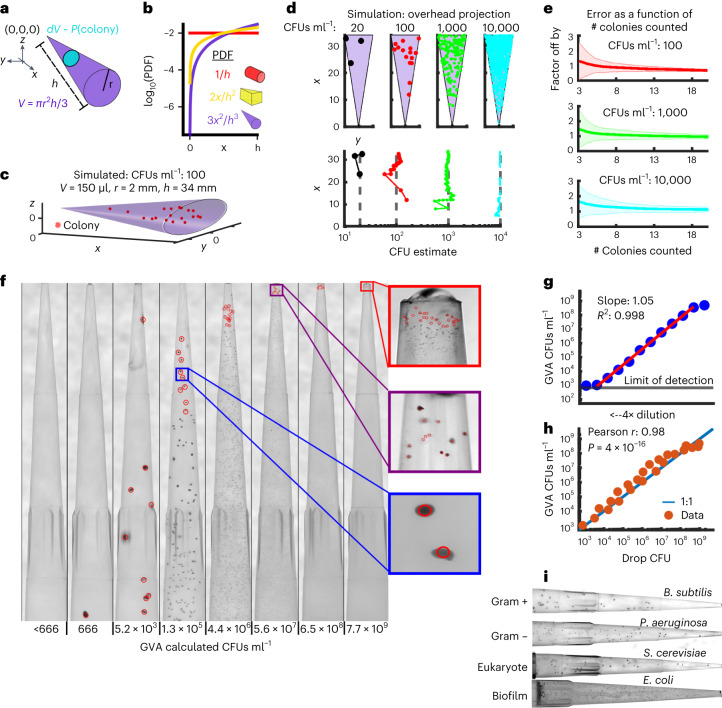
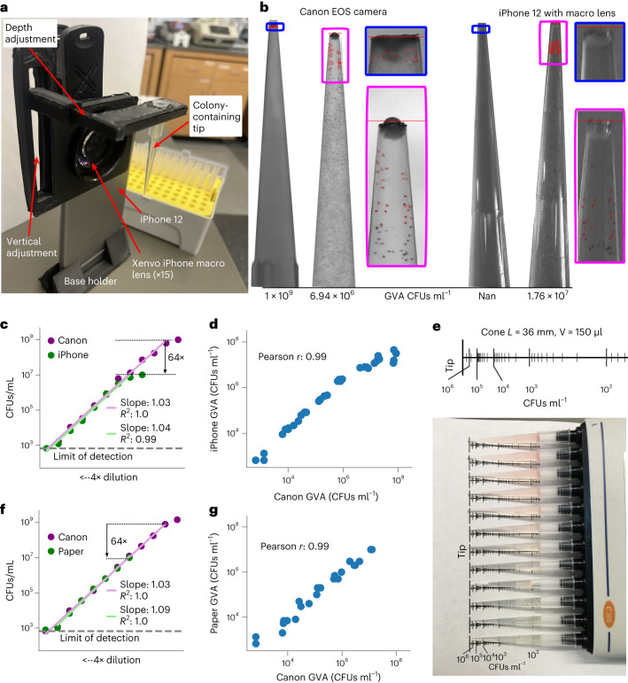
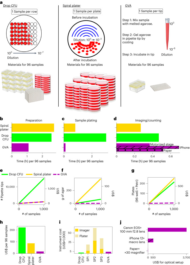
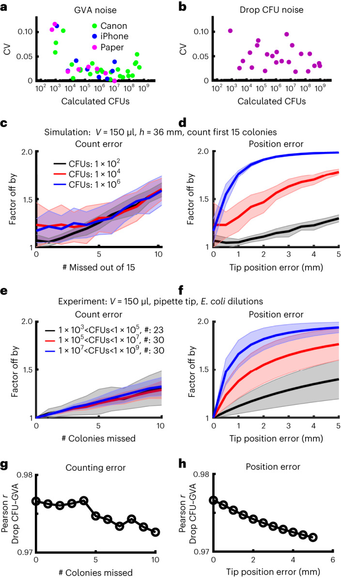
Counting viable cells is a universal practice in microbiology. The colony-forming unit (CFU) assay has remained the gold standard to measure viability across disciplines, but it is time-intensive and resource-consuming. Here we describe the geometric viability assay (GVA) that replicates CFU measurements over 6 orders of magnitude while reducing over 10-fold the time and consumables required. GVA computes a sample's viable cell count on the basis of the distribution of embedded colonies growing inside a pipette tip. GVA is compatible with Gram-positive and Gram-negative planktonic bacteria (Escherichia coli, Pseudomonas aeruginosa and Bacillus subtilis), biofilms and fungi (Saccharomyces cerevisiae). Laborious CFU experiments such as checkerboard assays, treatment time-courses and drug screens against slow-growing cells are simplified by GVA. The ease and low cost of GVA evinces that it can replace existing viability assays and enable viability measurements at previously impractical scales.

Fig. 1. The GVA.

a, The probability of a colony forming at a distance x from the tip of the cone is proportional to the infinitesimal volume dV (cyan circle) divided by the total volume V (purple cone). Analytically, this ratio is the probability density function (PDF) as a function of x (see Supplementary Information for derivation). b, The PDF for a cylinder (red), wedge (yellow) and cone (purple) as a function of the axial distance (x). c, Simulation of the colony distribution in a cone. d, Estimating the total CFUs ml⁻¹ on the basis of the position of colonies in the cone. Top: distributions of colonies for 4 simulations spanning 20 to 10,000 CFUs ml⁻¹ density. The volume of each cone is the same as in c. Bottom: GVA estimate of the CFUs ml⁻¹ as a function of the included colonies and their x positions. e, The factor the GVA calculation differs from the correct value as a function of the number of colonies in equation (1). Solid lines and shaded error bars represent mean ± 1s.d. of 1,000 simulations. Colours match simulations in d. f, Dilution series of E. coli embedded in 150 µl 0.5% LB agarose in p200 pipette tips. Red circles correspond to colonies counted using custom semi-automated segmentation software. CFUs ml⁻¹ estimates account for the initial 100× dilution of the sample into the agarose. g, E. coli CFUs ml⁻¹ calculated using GVA for a 4× dilution series. Points are the mean of 4 replicates, calculated after taking the log. The red line is the linear regression fit to the dilution series. A slope of 1 on a log–log plot is expected if the GVA estimate scales linearly with dilution. h, The drop CFU and GVA estimates are significantly correlated over 6 orders of magnitude. Four technical replicates were used for each sample for both methods. Significance assessed using Pearson r correlation. i, GVA performed on planktonic Gram-positive and Gram-negative bacteria, eukaryotic cells and bacterial biofilms (see Extended Data Fig. 4a for quantification).

Fig. 2. GVA dynamic range, but not accuracy, depends on the optical configuration.

a, Picture of assembled pipette tip holder on an iPhone 12 with a Xenvo macro lens. The pipette images were taken in front of a white backdrop (paper) with ambient illumination. b, Example images of the same 2 pipette tips using the Canon EOS with 100 mm f2.8 macro lens (left) or the iPhone 12 with Xenvo macro lens (right). The GVA-calculated CFUs ml⁻¹ are reported at the base of the tips. Selected colonies for GVA calculation are boxed. c, Dynamic range of the iPhone GVA. E. coli were diluted 4× and embedded in pipette tips. After incubation, the same tips were imaged with the iPhone camera with a macro lens (green) and the mirrorless camera (purple). Points are the average of 4 replicates calculated after taking the log. The green and purple lines are the linear regression fits to the dilution series. d, Pearson correlation between iPhone GVA and Canon camera for all pipettes where colonies could be counted using both. The correlation coefficient was calculated in log space. e, Top: ruler annotating the expected position of the 10th colony from the tip of a 36 mm, 150 µl cone for different concentrations of CFUs ml⁻¹. Bottom: paper-based GVA. f,g, Dynamic range (f) and correlation (g) of paper-based GVA measurements (green) to the Canon camera (purple). Points are the mean of 4 technical replicates.

Fig. 3. GVA reduces the time and materials for viability measurements by over 10-fold.

a, Left: schematic of a drop CFU assay and required materials for 96 samples assuming tips are changed for each dilution step. Middle: a spiral plater spreads a sample in an Archimedes spiral on a solid media plate. The spiral results in decreasing sample volume as a function of radial distance with a reported 3-log dynamic range. One Petri dish is required per sample. Right: GVA uses a single pipette tip to achieve a 6-order dynamic range. b–d, Time comparisons for different techniques. b, Time required to prepare solid growth media. c, Sample plating from a 96-well plate. d, Time required for quantification of 96 samples. e, Number and cost of pipette tips as a function of sample count for the three different techniques. See Supplementary Table 1 for cost estimates. f, Amount of agar required as a function of sample count. g, Number of 96-well plates and Petri dishes per condition. h, Estimated total cost in consumables per 96 samples using the three methods. GVA cost is US$0.17 per sample. i, Instrument costs. SP, spiral plater. j, The differences in instrumentation costs for the Canon, iPhone 12 and paper-based optical configurations.

Fig. 4. GVA has a low noise profile and is robust to missing colonies or tip position errors.

a,b, CV among 4 technical replicates for different CFU concentrations for GVA using the Canon, iPhone or paper optical configuration (a) and the drop CFU (b). Technical replicates were used to quantify the noise intrinsic to the technique. c,d, The factor by which GVA calculation differs from the correct value as a function of the number of missed colonies (c) or error in tip position (d) in simulated results (see Methods). Solid lines and shaded error bars depict the mean ± s.d. of 1,000 simulations. e,f, Same error calculations for experimental data. Solid lines and shaded error bars depict the mean ± s.d. of all the pipette tips (#) included in each bin. g,h, Correlation between the GVA and the drop CFU assay as a function of counting and position errors.

Extended Data Fig. 1. Derivation of a cone’s PDF.

a) The volume of the infinitesimal dV divided by the total volume V corresponds to the probability of finding a colony as a function of x. The radius of the infinitesimal (r'(x)) is a function of the radius of the cone′s base (r) divided by the height of the cone (h) times x according to trigonometry. b) The PDF of the cone as a function of x. The overhead projection of the cone is depicted above. c) The cumulative density function (CDF) as a function of x. d) The PDF is the same for axially symmetric cones such as square (red) and triangle (turquoise) pyramids. e) Two equivalent ways of calculating the number of CFUs in the wedge using either the CDF (left) or PDF (right). N(x) is the number of colonies counted. f) Percentage of simulations with the GVA calculated CFUs/mL within a factor of 2 of the correct value as a function of the number of colonies used for the GVA calculation. 1000 simulations were used to calculate the percentage. See Fig. 1c for simulation parameters. g) Examples of counting colonies in GVA. Red dots correspond to colonies. Cyan x’s are counted. Open circles are not counted, but their position is required for the integral. The left 2 panels are equivalent. The upper right panel is also correct but uses the CDF equation. The bottom right panel is incorrect as not all colonies were counted between x1 and x2.

Extended Data Fig. 2. Optical configuration.

a) CAD model showing the 3D printed optical box with lid (gray) holding pipette tips (green) attached to the base (purple). The base holds the glass plate, diffusion plate, and the LEDs used to illuminate the pipette tips in trans. b) Picture of optical configuration. The camera is mounted on a rail system perpendicular to a stepper motor rail with the optical box mounted. The GVA samples are positioned using a 12-channel pipetter held in position with the optical box lid and imaged using a Canon EOS RP camera with an f/2.8 100 mm macro lens. The electronics box houses the circuitry required to control the LEDs and stepper motor. An Arduino Uno is used to control both which interfaces with the MATLAB application used to segment the pipette tip images (see Methods). c) Pixel resolution for this configuration is 6.65 microns.

Extended Data Fig. 3. Example drop CFU plate and Bland-Altman analysis.

a) Each sample (columns) is diluted with a 10-fold serial dilution (rows) and 3 µL are spotted on a 1.5% LB agar pad. Colonies are counted for the dilution row where individual colonies are discrete. These counts are used to calculate the CFUs/mL (bottom). b) Bland-Altman plot comparing GVA and drop CFU measurements. CFU values were log-transformed for the comparison. The method difference (Δ) as a function of the mean of the methods (x-axis) was fit using a linear regression model (red line, equation) with confidence intervals depicted (dotted red lines). The limits of agreement, equal to 1.96X the standard deviation in Δ between the methods is depicted in the black dotted lines. The bias, equal to the mean Δ across the data is annotated in the solid black line.

Extended Data Fig. 4. GVA calculations for different species.

a) For the six species tested with GVA, the average number of CFUs/mL between 3 biological replicates for different dilution series. Error bars represent the standard deviation between replicates. b) Plates streaked with pipette tip after GVA embedding before or after bleach wash. No change in CFUs/mL was observed after a bleach wash. c) Biofilm growth over time. Error bars correspond to the standard deviation between 6 biological replicates and points represent the mean. d) Mean GVA using Low Melt Agar quantifying a dilution series of E. coli cells between 3 biological replicates. Error bars represent the standard deviation between replicates. e) GVA in blood agar (5% sheeps blood) with E. coli cells. f) Example tips from with blood agar showing E. coli colonies. Colonies stained with TTC.

Extended Data Fig. 5. Square pyramid version of GVA.

a, b) 3D printed molds for creating square pyramid for 12 (a) and 48 (b) conditions. c) Picture of a 9x dilution series of E. coli cultures on the GVA chip. d) GVA calculated CFUs/mL using for a dilution series. Each dot is the mean of 4 technical replicates. e) The noise is measured using the coefficient of variation (COV) for the chip GVA. f) Matched drop CFU quantification to conditions in (d). g) Corresponding noise analysis for drop CFU. The error bars represent the standard deviation between 4 technical replicates. h) Correlation between chip GVA and drop CFU over 5 orders of magnitude. The error bars represent the standard deviation between 4 technical replicates. Significance assessed using Pearson correlation. i, j) Chip GVA for Gram-positive (i) and eukaryotic (j) cells.

Extended Data Fig. 6. Biome sampling using GVA.

a) Twenty-four positions (red dots) on a volunteer were swabbed vigorously for 15 seconds before being placed in 1 mL of LB medium and vortexed for 10 seconds. 50 µL of the sample was then mixed with 150 µL of 0.66% melted LB agar to a final concentration of 0.5% agar and allowed to gel in the tips. With this protocol, the lower limit of detection was 20 CFUs/mL (dotted line). The sample replicates were incubated at 30 °C or 25 °C for 48 hours before imaging. Error bars denote the standard deviation between 3 biological replicates and bars the mean. b) Example pipette tips for different sample regions reveals diverse colony structure and concentration for different biome locations. All samples were stained with TTC. c) Samples from higher thermal regions (ear, armpit) grew at 30 °C but did not grow at 25 °C indicating the temperature selectivity of different species grown in the pipette tip.

Extended Data Fig. 7. iPhone pipette tip holder.

a) The 3D printed parts for stereotypically positioning a pipette tip in front of an iPhone rear camera with a Xenvo macro lens (15x magnification without the widefield lens). The blue face plate slides onto the Xenvo macro lens which is clipped to the iPhone. The green bar is attached with a screw to the side channel on the blue plate. This allows for adjusting the height by sliding the green bar in the channel. The purple extension bar slides into the green channel to adjust the imaging depth. b) The phone is held upright with a stand (yellow). Pieces printed with standard FDM printing with PLA.

Extended Data Fig. 8. Sensitivity analysis of GVA calculations to error in missing colonies and location of the tip.

a) Heatmap of the error as a function of both tip position and missing colony errors. b) Same analysis as in panel a, but with experimental data. CFUs/mL binned between 1e3 and 1e5 (top row), 1e5 and 1e7 (middle row), and 1e7 to 1e9 (bottom row). The number of pipette tips included in each bin is annotated by the count. c) Heatmap of the Pearson correlation between the drop CFU and GVA for both tip position and missing colony errors.

References

1. Lázár, V., Snitser, O., Barkan, D. & Kishony, R. Antibiotic combinations reduce Staphylococcus aureus clearance. Nature10.1038/s41586-022-05260-5 (2022). - PMC - PubMed
1. Zheng EJ, Stokes JM, Collins JJ. Eradicating bacterial persisters with combinations of strongly and weakly metabolism-dependent antibiotics. Cell Chem. Biol. 2020;27:1544–1552.e3. doi: 10.1016/j.chembiol.2020.08.015. - DOI - PubMed
1. Hazan R, Que YA, Maura D, Rahme LG. A method for high throughput determination of viable bacteria cell counts in 96-well plates. BMC Microbiol. 2012;12:259. doi: 10.1186/1471-2180-12-259. - DOI - PMC - PubMed
1. Thieme L, et al. Adaptation of the start-growth-time method for high-throughput biofilm quantification. Front. Microbiol. 2021;12:2395. doi: 10.3389/fmicb.2021.631248. - DOI - PMC - PubMed
1. Otašević S, et al. Non-culture based assays for the detection of fungal pathogens. J. Mycol. Med. 2018;28:236–248. doi: 10.1016/j.mycmed.2018.03.001. - DOI - PMC - PubMed
LinkOut - more resources