Unified topological inference for brain networks in temporal lobe epilepsy using the Wasserstein distance

Abstract

Persistent homology offers a powerful tool for extracting hidden topological signals from brain networks. It captures the evolution of topological structures across multiple scales, known as filtrations, thereby revealing topological features that persist over these scales. These features are summarized in persistence diagrams, and their dissimilarity is quantified using the Wasserstein distance. However, the Wasserstein distance does not follow a known distribution, posing challenges for the application of existing parametric statistical models. To tackle this issue, we introduce a unified topological inference framework centered on the Wasserstein distance. Our approach has no explicit model and distributional assumptions. The inference is performed in a completely data driven fashion. We apply this method to resting-state functional magnetic resonance images (rs-fMRI) of temporal lobe epilepsy patients collected from two different sites: the University of Wisconsin-Madison and the Medical College of Wisconsin. Importantly, our topological method is robust to variations due to sex and image acquisition, obviating the need to account for these variables as nuisance covariates. We successfully localize the brain regions that contribute the most to topological differences. A MATLAB package used for all analyses in this study is available at https://github.com/laplcebeltrami/PH-STAT.

Fig. 1.

The average correlation brain networks of 50 healthy controls (HC) and 101 temporal lobe epilepsy (TLE) patients. They are overlaid on top of the gray matter boundary of the MNI template. The brain network of TLE is far sparse compared to that of HC. The sparse TLE network is also consistent with the plot Betti-0 curve where TLE networks are more disconnected than HC networks. It demonstrates the global dysfunction of TLE and the breakdown of typical brain connectivity.

Fig. 2.

Graph filtrations are obtained by sequentially thresholding graphs in increasing edge weights. The 0th Betti number ${\beta }_0$ (number of connected components) and the first Betti number ${\beta }_1$ (number of cycles) are then plotted over the filtration values. The Betti curves are monotone over graph filtrations. However, different graphs (top vs. middle) can yield identical Betti curves. As the number of nodes increases, the chance of obtaining the identical Betti curves exponentially decreases. The edges that increase ${\beta }_0$ (red) forms the birth set while the edge that decrease ${\beta }_0$ (blue) forms the death set. The birth and death sets partition the edge set.

Fig. 3.

The comparison between the Rips and graph filtrations performed on 50 scatter points randomly sampled in a unit cube. The Euclidean distance between points are used as edge weights. Unlike Rips filtrations, ${\beta }_0$ and ${\beta }_1$ curves for graph filtrations are always monotone making the subsequent statistical analysis far more stable.

Fig. 4.

Betti-0 and Betti-1 curves obtained in graph filtrations on 50 healthy controls (HC) and 101 temporal lobe epilepsy (TLE) patients. TLE has more disconnected subnetworks $\left({\beta }_0\right)$ compared to HC while having compatible higher order cyclic connectivity $\left({\beta }_1\right)$. The statistical significance of Betti curve shape difference is quantified through the proposed Wasserstein distance.

Fig. 5.

The birth and death sets of 50 healthy controls (HC) and 101 temporal lobe epilepsy (TLE) patients. The Wasserstein distance between the birth sets measures 0D topology difference while the Wasserstein distance between the death sets measures 1D topology difference.

Fig. 6.

Maximum spanning trees (MST) of the average correlation of HC and TLE. MST are the 0D topology while none-MST edges not shown here are 1D topology. MST forms the birth set. MST of rs-fMRI is mainly characterized by the left-right connectivity.

Fig. 7.

Pairwise Wasserstein distance between 50 healthy controls (HC) and 101 temporal lobe epilepsy (TLE) patients. There are subtle pattern difference in the off-diagonal patterns (between group distances ${ℒ}_B$) compared to diagonal patterns (within group distances ${ℒ}_W$). The permutation test with 100 million permutations was used to determine the statistical significance using the ratio statistic. The red line is the observed ratio. The histogram is the empirical null distribution obtained from the permutation test.

Fig. 8.

The plot of ratio statistic ${\varphi }_{ℒ}$ (top) over 100 million transpositions in testing the topological difference between HC and TLE. The plot is only shown at every 10000 transposition. The redline is the observed ratio static 0.9541. The estimated $p$-value (middle) converges to 0.0086 after 100 million transpositions. The CPU time (bottom) is linear and takes 102 s for 100 million transpositions.

Fig. 9.

Simulation study testing topological equivalence (top) and difference (bottom) in three noise settings: $\sigma =0.1$ (left), 0.2 (middle), 0.3 (right). We should not cluster topologically equivalent patterns while we should cluster topologically different patterns well.

Fig. 10.

Left: Topological embedding of 151 subjects. Green circles are HC and yellow circles are TLE. The blue square is the topological center of HC while the red square is the topological center of TLE. The horizontal axis represents 0D topology (connected components) through birth values while the vertical axis represents 1D topology (circles) through death values. The embedding shows that the topological separation is mainly through 0D topology. Right: Embedding through graph theory features global efficiency at vertical and Q-modularity at horizontal axes.

Fig. 11.

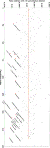
The plot of the Wasserstein distance based ratio static ${\varphi }_{ℒ}$ under the node attack. The red line is the ratio statistic of the whole brain network without any node attack. After deleting each parcellation under the node attack, we recomputed the ratio statistic (black dots). The biggest drop in the ratio statistic corresponds to the biggest topological difference for TLE. Listed 20 regions that decrease the ratio statistic and in turn decreases the discrimination power the most.

Fig. 12.

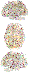
20 localized brain regions (teal color) identified under node attack on the ratio statistic ${\varphi }_{ℒ}$ displayed over Glasser pacellated brain regions. The results are overlaid on top of average correlation map of TLE patients.

Fig. 13.

The ratio ${\psi }_l$ of the within-cluster distance over the between-cluster distance. The topological approach using the Wasserstein distance usually gives far smaller ratio compared to the traditional $k$-means clustering. In the elbow method, the largest slope change occurs at $k=3$ and we determine $k=3$ is the optimal number of clusters.

Fig. 14.

Schematic of Theorem 6 with 4-nodes examples. Each step of operations yield graphs with valid birth–death decompositions. The first row is the construction of sum operation by projecting to $W_1$. The second row is the construction of sum operation by projecting to $W_2$. Red colored edges are the maximum spanning trees (MST). Each addition operation will not change MST. Eventually, we can have two different graphs with the identical birth–death decomposition.

References

1. Abdallah H, Regalski A, Kang MB, Berishaj M, Nnadi N, Chowdury A, Diwadkar VA, Salch A, 2023. Statistical inference for persistent homology applied to simulated fMRI time series data. Found. Data Sci 5, 1–25.
1. Adamovich T, Zakharov I, Tabueva A, Malykh S, 2022. The thresholding problem and variability in the EEG graph network parameters. Sci. Rep 12, 18659. - PMC - PubMed
1. Adams H, Emerson T, Kirby M, Neville R, Peterson C, Shipman P, Chepushtanova S, Hanson E, Motta F, Ziegelmeier L, 2017. Persistence images: A stable vector representation of persistent homology. J. Mach. Learn. Res 18, 218–252.
1. Adler RJ, Bobrowski O, Borman MS, Subag E, Weinberger S, 2010. Persistent homology for random fields and complexes. In: Borrowing Strength: Theory Powering Applications-a Festschrift for Lawrence D. Brown Institute of Mathematical Statistics, pp. 124–143.
1. Agueh M, Carlier G, 2011. Barycenters in the wasserstein space. SIAM J. Math. Anal 43, 904–924.
Publication types