Earlier and more uniform spring green-up linked to lower insect richness and biomass in temperate forests

Abstract

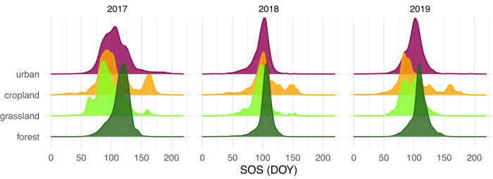
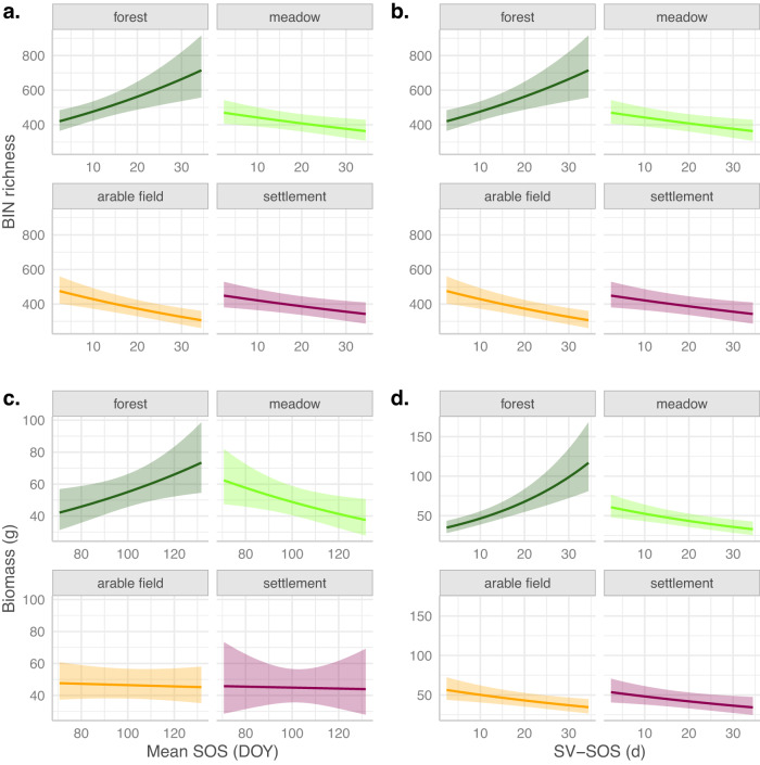
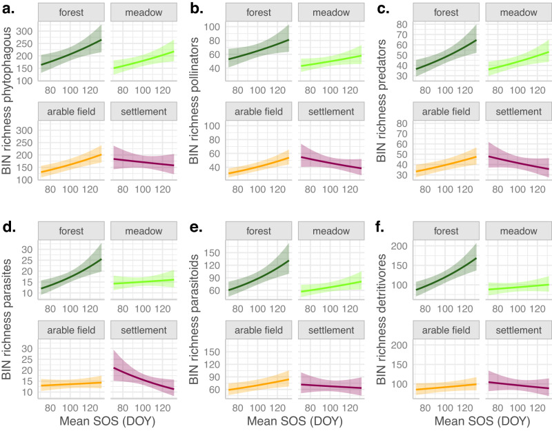
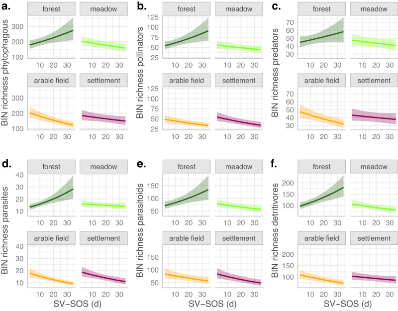
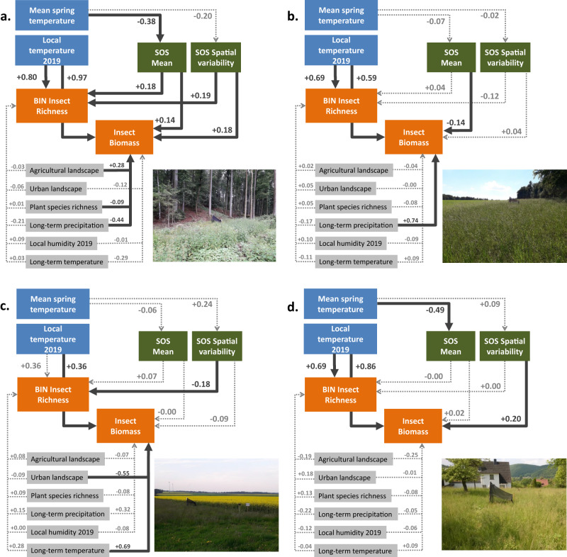
Urbanization and agricultural intensification are considered the main causes of recent insect decline in temperate Europe, while direct climate warming effects are still ambiguous. Nonetheless, higher temperatures advance spring leaf emergence, which in turn may directly or indirectly affect insects. We therefore investigated how Sentinel-2-derived start of season (SOS) and its spatial variability (SV-SOS) are affected by spring temperature and whether these green-up variables can explain insect biomass and richness across a climate and land-use gradient in southern Germany. We found that the effects of both spring green-up variables on insect biomass and richness differed between land-use types, but were strongest in forests. Here, insect richness and biomass were higher with later green-up (SOS) and higher SV-SOS. In turn, higher spring temperatures advanced SOS, while SV-SOS was lower at warmer sites. We conclude that with a warming climate, insect biomass and richness in forests may be affected negatively due to earlier and more uniform green-up. Promising adaptation strategies should therefore focus on spatial variability in green-up in forests, thus plant species and structural diversity.

Fig. 1. SOS distribution per year and land use type.

Annual density ridges of SOS (DOY) in 2017-2019 for the four most dominant land use types (covering 99.99% of nonwater surface) in 100 m radii around the 179 study plots with Malaise traps on a climate and land-use gradient in Bavaria. “Semi-natural areas” (covering 0.01% of non-water surface) are not shown.

Fig. 2. Partial effects of the green-up variables on insect BIN richness and Biomass.

Effects were derived from generalized additive models (gams) on BIN richness (a, b) and on Biomass (c, d), in which we included regional land use and interactions of local land use with all green-up variables, with all climate variables and with species richness as fixed linear effects (see Table 1). ‘Day’ was used as smoothed effect and space as random effect. An offset of log(sampling days) was used to control for sampling period differences. For biomass, family = gaussian(link = “log”) and for richness, family = negative binomial were used. Insect data were recorded over a whole season (8 samplings) at 179 traps, resulting in 1214 observations for BIN Richness and 1293 observations for Biomass. a, c, partial effects of mean SOS. b, d, partial effects of SV-SOS.

Fig. 3. Partial effect plots of mean SOS in interaction with local land use on BIN richness per functional group.

Effects were derived from generalized additive models (gam) in which we included regional land use and interactions of local land use with all green-up variables, with all-climate variables and with species richness as fixed linear effects. As in the initial model (Fig. 2, Table 1) ‘Day’ was used as smoothed effect and space as random effect. An offset of log(sampling days) was used to control for sampling period differences. Family = negative binomial was used. Insect data were recorded over a whole season (8 samplings at 179 traps), resulting in 1214 observations per model. a, phytophagous insects. b, pollinators. c, predators. d, parasites. e, parasitoids. f, detritivores.

Fig. 4. Partial effect plots of SV-SOS in interaction with local land use on BIN richness per functional group.

Effects were derived from generalized additive models (gam) in which we included regional land use and interactions of local land use with all green-up variables, with all-climate variables and with species richness as fixed linear effects. As in the initial model (Fig. 2, Table 1), ‘Day’ was used as smoothed effect and space as random effect. An offset of log(sampling days) was used to control for sampling period differences. Family = negative binomial was used. Insect data were recorded over a whole season (8 samplings at 179 traps), resulting in 1214 observations per model. a, phytophagous insects. b, pollinators. c, predators. d, parasites. e, parasitoids. f, detritivores.

Fig. 5. Confirmatory path models for each local land-use type.

a, forest. b, meadow. c, arable field. d, settlement. Each confirmatory path model contains two components: one part using linear models to explain green-up variables by mean spring temperature. In forests, n = 55 per model, in meadows, n = 45 per model, in arable fields, n = 44 per model, in settlements, n = 35 per model; the other part using generalized additive models to explain BIN richness and biomass by the green-up variables, climate variables, regional land use and plant species richness as fixed linear effects. As in the initial model (Fig. 2, Table 1), ‘Day’ was used as smoothed effect and space as random effect. Instead of offsets of log(sampling duration), log(richness)/log(sampling duration) and log(biomass)/log(sampling duration) were used to control for sampling period differences. For biomass, family = gaussian(link = “log”) and for richness, family = negative binomial was used. In forest plots, n = 376 for richness and n = 395 for biomass, in meadows, n = 310 for richness and n = 333 for biomass, in arable fields, n = 298 for richness and n = 313 for biomass. In settlement plots, n = 230 for richness and n = 252 for biomass. Numbers indicate standardized partial effects. Dark grey thick arrows indicate significant paths (p < 0.05), light grey insignificant paths. Pictures show Malaise trap plots in each of the local land-use types.

References

1. Hallmann CA, et al. More than 75 percent decline over 27 years in total flying insect biomass in protected areas. PloS One. 2017;12:e0185809. - PMC - PubMed
1. Costanza R, et al. The value of the world’s ecosystem services and natural capital. Nature. 1997;387:253–260.
1. Uhler J, et al. Relationship of insect biomass and richness with land use along a climate gradient. Nat. Commun. 2021;12:5946. - PMC - PubMed
1. Habel JC, Ulrich W, Biburger N, Seibold S, Schmitt T. Agricultural intensification drives butterfly decline. Insect Conserv. Diversity. 2019;12:289–295.
1. Fenoglio MS, Rossetti MR, Videla M. Negative effects of urbanization on terrestrial arthropod communities: A meta‐analysis. Glob. Ecol. Biogeogr. 2020;29:1412–1429.
Publication types