Truly pattern: Nonlinear integration of motion signals is required to account for the responses of pattern cells in rat visual cortex

Abstract

A key feature of advanced motion processing in the primate dorsal stream is the existence of pattern cells-specialized cortical neurons that integrate local motion signals into pattern-invariant representations of global direction. Pattern cells have also been reported in rodent visual cortex, but it is unknown whether the tuning of these neurons results from truly integrative, nonlinear mechanisms or trivially arises from linear receptive fields (RFs) with a peculiar geometry. Here, we show that pattern cells in rat primary (V1) and lateromedial (LM) visual cortex process motion direction in a way that cannot be explained by the linear spatiotemporal structure of their RFs. Instead, their tuning properties are consistent with and well explained by those of units in a state-of-the-art neural network model of the dorsal stream. This suggests that similar cortical processes underlay motion representation in primates and rodents. The latter could thus serve as powerful model systems to unravel the underlying circuit-level mechanisms.

Fig. 1.. Illustration of how blobby, linear receptive fields can produce tuning consistent with the behavior of pattern cells.

(A) Left: Spatial structure of the linear filters used to simulate receptive field (RFs) with progressively lower aspect ratio (from top to bottom) using Gabor functions. Right: Tuning curves showing the selectivity for grating and plaid direction (dashed and solid lines, respectively) of the linear filters shown on the left. (B) Cartoon of an elongated RF with high aspect ratio that poorly matches the local contrast features of a plaid drifting at 135° (orange arrow), made of two superimposed gratings drifting at 90° and 210° (green arrows). When the orientation of the RF is orthogonal to the local direction of one of the constituent gratings (bottom/right), there will be times at which the average luminance falling within the subunits of the RF matches their polarity, producing a strong response. If instead the RF is orthogonal to the global direction of the plaid (top/left), the average luminance falling within each RF subunit is approximately mid-gray, producing no response. The unit can thus signal the local direction of the grating (thick green arrow) but not the global direction of the plaid (thick orange arrow). (C) Cartoon of a blobby RF with low aspect ratio that matches well the local contrast features of the plaid [same stimulus as in (B)]. Regardless whether the RF is orthogonal to the local direction of the constituent gratings (bottom/right) or to the global direction of the plaid (top/left), there will be times at which the average luminance falling within the RF subunits matches their polarity, producing strong responses. The unit will thus respond similarly to gratings and plaids drifting along the same direction, yielding the pattern-cell tuning shown in (A) (bottom plot). Cartoons in (A) and (B) are inspired from (17).

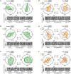
Fig. 2.. Examples of pattern and component cells recorded in areas V1, LM, and RL.

Each panel depicts the observed tuning curves (i.e., normalized average response for each stimulus direction) for gratings (left; solid line) and plaids (right; solid line), as well as the tuning curves predicted by an LN model based on the spatiotemporal filter estimated via STA (dashed lines). The pairs of values Z_c and Z_p and Z_c′ and Z_p′ are the component and pattern indexes computed for the observed and predicted tuning curves, respectively. The temporal sequence of STA images at different time lags preceding spike generation is also shown (bottom), along with the CI values that quantify the sharpness of each STA filter. In every STA image, each pixel intensity value was independently z-scored, based on the null distribution of STA values obtained through a permutation test (see Supplementary Text). A gray-scale map was used to visualize the resulting z-scored values within the [−6, +6] range (see scale bars). (A) Sharply tuned component cell from V1, correctly predicted by the LN model as component. (B) Sharply tuned component cell from LM, correctly predicted by the LN model as component. (C) Broadly tuned component cell from V1, correctly predicted by the LN model as component. (D) Sharply tuned pattern cell from LM, incorrectly predicted by the LN model as unclassified. (E and F) Sharply tuned pattern cells from LM, incorrectly predicted by the LN model as component.

Fig. 3.. Distribution of pattern and component cells in areas V1, LM, and RL.

(A to C) Scatter plots showing the distributions of the pairs of observed Z_p and Z_c indexes for the cells recorded in the three targeted areas. Light-colored dots represent units not meeting the direction selectivity criterion (i.e., DSI > 0.33); dark-colored dots represent units meeting such criterion. Dashed lines are decision boundaries in the Z_p/Z_c plane that distinguish regions where cells are labeled as component (in green; bottom-right corner), pattern (in orange; top-left corner), or unclassified (in gray; central area). (D) Schematic map of rat visual cortex showing the anatomical locations of V1, LM, and RL. (E) Percentage of component cells (green bars) and pattern cells (orange bars) recorded in V1 (left), LM (center), and RL (right). (F) Distributions of cross-orientation suppression index (CSI) values across area-pooled populations of component (left; green), pattern (center; orange), and unclassified (right; gray) units. All medians were significantly larger than zero (***P < 0.001, Wilcoxon test). The medians of the component and pattern cells’ pools were not statistically different from each other (P > 0.05, Wilcoxon test). n.s., nonsignificant.

Fig. 4.. Component cells have sharper and more Gabor-like, linear RFs than pattern cells.

(A) Representative examples of STA images obtained for nine component cells (top, green frames) and nine pattern cells (bottom, orange frames). Each image is shown along with the corresponding CI and a metric (R²) that quantifies the GOF with a Gabor function. For each neuron, the RF shown here is taken at the time before spike generation when the number of distinct subfields (lobes) was the largest. (B) Distributions of CI values of the STA images obtained for the area-pooled populations of component (left, green), pattern (center, orange), and unclassified (right, gray) units at all tested (10) time lags from spike generation. All units in the proper quadrants of the Z_c/Z_p plane, with no constraint on direction selectivity, were included in this analysis (i.e., all green, orange, and gray dots of Fig. 3, A to C, were used, no matter whether light or dark). The median CIs of component and pattern cells were significantly different according to a Wilcoxon test (***P = 0.003). (C) Same as in (B), but for the distributions of R² values (assessing the GOF with a Gabor function), whose medians were significantly different, for the component and pattern cells, according to a Wilcoxon test (*P = 0.03). (D) Distribution of the number of distinct lobes in the STA image (binarized at 3.5σ) with the largest CI obtained for the component (green bars) and pattern (orange bars) cells shown in Fig. 3, A to C, [as in (B) and (C), no constraint was imposed on the level of direction selectivity]. The distributions were statistically different according to a χ² test (P = 0.047).

Fig. 5.. Linear RFs do not account for global motion selectivity of pattern cells.

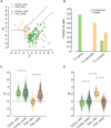
(A) Scatter plot showing the distributions of the pairs of observed Z_p and Z_c indexes for pattern (light orange) and component cells (light green) recorded across V1, LM, and RL together with the values of the same indexes (dark orange and green dots), when computed on the tuning curves predicted using the spatiotemporal RFs that were estimated via STA. The lines connect the observed and predicted pairs of index values to highlight the displacement in the Z_p/Z_c plane for each unit. Same layout and color code as in Fig. 3, A to C. (B) Bar plot reporting the fraction of units (pattern cells in orange and component cells in green) that preserved their original classification (left; “To same” label), switched to the opposite class (center; “To opposite” label), or landed in the unclassified region (right: “To unclass.” label), when the Z_p and Z_c indexes were computed on the predicted direction tuning curves. (C) Distributions of observed (light colors) and predicted (dark colors) Z_c values for the two populations of component (green) and pattern (orange) cells. (D) Distributions of observed (light colors) and predicted (dark colors) Z_p values for the two populations of component (green) and pattern (orange) cells. In (C) and (D), the statistical comparison between the medians of the observed versus predicted distributions for the same neuronal populations was performed using a paired Wilcoxon test (**P < 0.01; ***P < 0.001). In (D), the statistical comparison between the median of the predicted Z_p indexes for the component cells versus the median of the observed Z_p indexes for the pattern cells was carried out using an unpaired Wilcoxon test (**P < 0.01).

Fig. 6.. Phase invariance of component and pattern cells.

(A) Response dynamics of two example component cells (left, green) and pattern cells (right, orange), following presentation of the most effective grating. Each panel depicts (i) the observed, normalized tuning curves for gratings (light color; the black dot indicates the response to the preferred grating) and plaids (dark color); (ii) the raster plot, with the times at which individual action potentials were fired across repeated presentations of the most effective grating, as well as the resulting peristimulus time histogram (PSTH), computed in 10-ms-wide time bins, which reports the normalized, trial-averaged firing rate of the neuron during stimulus presentation (stimulus onset and offset are marked by the vertical dashed lines); and (iii) the power spectrum of the PSTH, with its mean (horizontal gray line), its mean ± SD (dashed lines), and the TF of the grating (vertical gray line; the black dot marks the value of the power spectrum at the stimulus frequency). The value of the MI (defined in Materials and Methods) is also reported for each example cell. (B) Distributions of MI values for the populations of component (in green) and pattern (in orange) cells, as computed from the response to the most effective grating for each unit. The dashed line indicates the conventional threshold to distinguish simple (MI > 3) from complex cells (MI < 3). The median MI was slightly but significantly higher for component than for pattern cells (P < 0.05, Wilcoxon test). (C) Bar plot reporting the fraction of cells in each population being classified as complex cells (i.e., having MI < 3). Although this fraction was larger for pattern than for component cells, the difference did not reach statistical significance (P > 0.05, χ² test).

Fig. 7.. The units of DorsalNet display tuning properties that are highly consistent with those observed for rat visual cortical neurons.

(A and B) Examples of DorsalNet units displaying the typical tuning of a component cell (A) and of a pattern cell (B). Same layout and color code used in Fig. 2. (C) Schematic of DorsalNet layer structure. (D) Fraction of component (green bars), pattern (orange bars), and unclassified (gray bars) units from layer #0 to layer#5 of DorsalNet (compare to Fig. 3E). (E) Distribution of CSI values for component (green), pattern (orange), and unclassified (gray) units, pooled across all DorsalNet layers (same layout, color code, and statistical analysis as in Fig. 3F). (F and G) Distribution of CI and R² values for component (green), pattern (orange), and unclassified (gray) units (same layout, color code, and statistical analysis as in Fig. 4, B and C). (H) Scatter plot showing (i) the distribution of observed Z_p and Z_c indexes for pattern (light orange) and component (light green) units, pooled across all DorsalNet layers, and (ii) the values of the same indexes (dark orange and green), as computed for the tuning curves predicted using the spatiotemporal RFs that were estimated via STA (compare to Fig. 5A). (I and J) Distributions of observed (light colors) and predicted (dark colors) Z_c and Z_p values for the populations of DorsalNet units classified as component (green) and pattern (orange; same layout, color code, and statistical analysis as in Fig. 5, C and D). (K) Bar plot showing the fraction of DorsalNet units that preserved their original classification, switched to the opposite class, or became unclassified (same layout and color code as in Fig. 5B), when the Z_p and Z_c indexes were computed on the predicted direction tuning curves. The analyses in (E) to (K) refer to units of the same class, pooled across all DorsalNet layers, respectively.

Fig. 8.. DorsalNet component and pattern units account for the tuning of matching populations of rat visual cortical neurons.

(A) Left: Normalized responses of rat component cells, as a function of grating (left matrix) and plaid (right matrix) direction (the cells have been ordered based on the direction of their preferred grating). Right: Population averages of the direction tuning curves for gratings (light green) and plaids (dark green), with the resulting Z_c, Z_p, and PI indexes. Before averaging, each curve has been realigned to center the direction of the preferred grating of the cell on zero. (B and C) Same as in (A), but for the predicted (rather than measured) responses of rat component cells, as obtained by linear models using the activations of DN component (B) and pattern (C) units as regressors. (D) Same as in (A), but for the measured direction tuning curves of rat pattern cells. (E and F) Same as in (B) and (C), but for the predicted responses of rat pattern cells. (G) Bar plot displaying the error (cross-validated, population-averaged RMSE) in predicting the tuning for grating and plaid direction for the populations of component (green) and pattern (orange) cells, using the activations of DN component, pattern, and unclassified units, as well as the STA-based LN model. Error bars indicate the SE. Statistical comparisons between average RMSEs were performed using an unpaired t tests (*P < 0.05, **P < 0.01, and ***P < 0.001). (H and I) Same analyses as in Fig. 5 (C and D) and Fig. 5A, but for the predictions obtained by using the activations of DN component units. (J and K) Same as in (H) and (I), but with the predicted Z_c and Z_p indexes obtained by using DN pattern units as regressors. (L and M) Same analysis as in Fig. 5B, but for the predictions yielded by DN component (I) and pattern (K) regressors, respectively.

Fig. 9.. Unclassified cells behave as a qualitatively distinct population from pattern and component cells, when investigated through DorsalNet modeling.

(A) Bar plot displaying the error in predicting the tuning for grating and plaid direction for the population of unclassified cells [same four models and statistical tests as in (G)]. (B) Fraction of component (green), pattern (orange), and unclassified (gray) cells for which the best DorsalNet prediction (i.e., lowest RMSE) was obtained by the matching population of DN units. (C) Scatter plot showing the distributions of the pairs of observed Z_p and Z_c indexes for the component, pattern, and unclassified cells (same data of Fig. 3, A to C, but pooled across areas). The outer color of each dot shows the original classification, based on the Z_p and Z_c values (green: component; orange: pattern; black: unclassified). The inner color reports which population of DN units better predicted the tonging of the cell (green: component DN units; orange: pattern DN units; black: unclassified DN units). (D) Confidence of the best-fitting DorsalNet models in predicting the tuning of rat cortical neurons. Confidence scores (see Supplementary Text for a definition) are plotted separately for the three classes of component (green), pattern (orange), and unclassified (gray) cells (which population of DN units best fitted the tuning is not indicated in this plot). Statistical differences were assessed using an unpaired Wilcoxon tests (***P < 0.001). (E) Same as in Fig. 8A, but for the two populations of unclassified cells for which DN component units (left plots) and DN pattern units (right plots) yielded the most accurate prediction of their direction tuning curves (i.e., predictions with confidence score > 0.3). These two populations are referred to as “quasi-pattern” or “quasi-component” in the main text.

References

1. D. Marr, Vision: A Computational Investigation into the Human Representation and Processing of Visual Information (MIT Press, 2010).
1. C. L. Fennema, W. B. Thompson, Velocity determination in scenes containing several moving objects. Comput. Graph. Image Process. 9, 301–315 (1979).
1. S. Wüerger, R. Shapley, N. Rubin, “On the visually perceived direction of motion” by Hans Wallach: 60 years later. Perception 25, 1317–1367 (1996).
1. J. A. Movshon, E. H. Adelson, M. S. Gizzi, W. T. Newsome, C. Chagas, R. Gattass, C. Gross, Pattern Recognition Mechanisms (Springer-Verlag, 1985).
1. H. R. Rodman, T. D. Albright, Single-unit analysis of pattern-motion selective properties in the middle temporal visual area (MT). Exp. Brain Res. 75, 53–62 (1989). - PubMed