How Robust Is the Ligand Binding Transition State?

Abstract

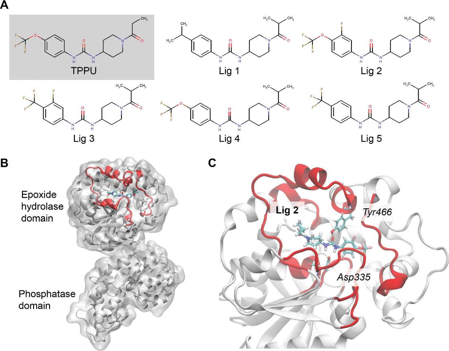
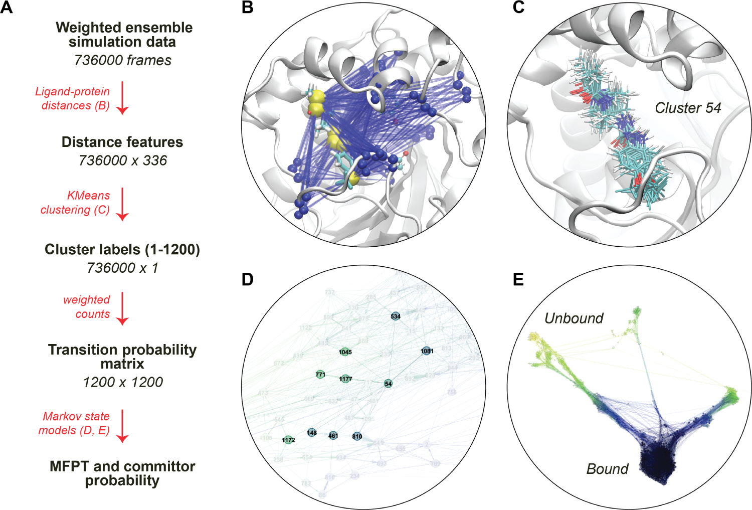
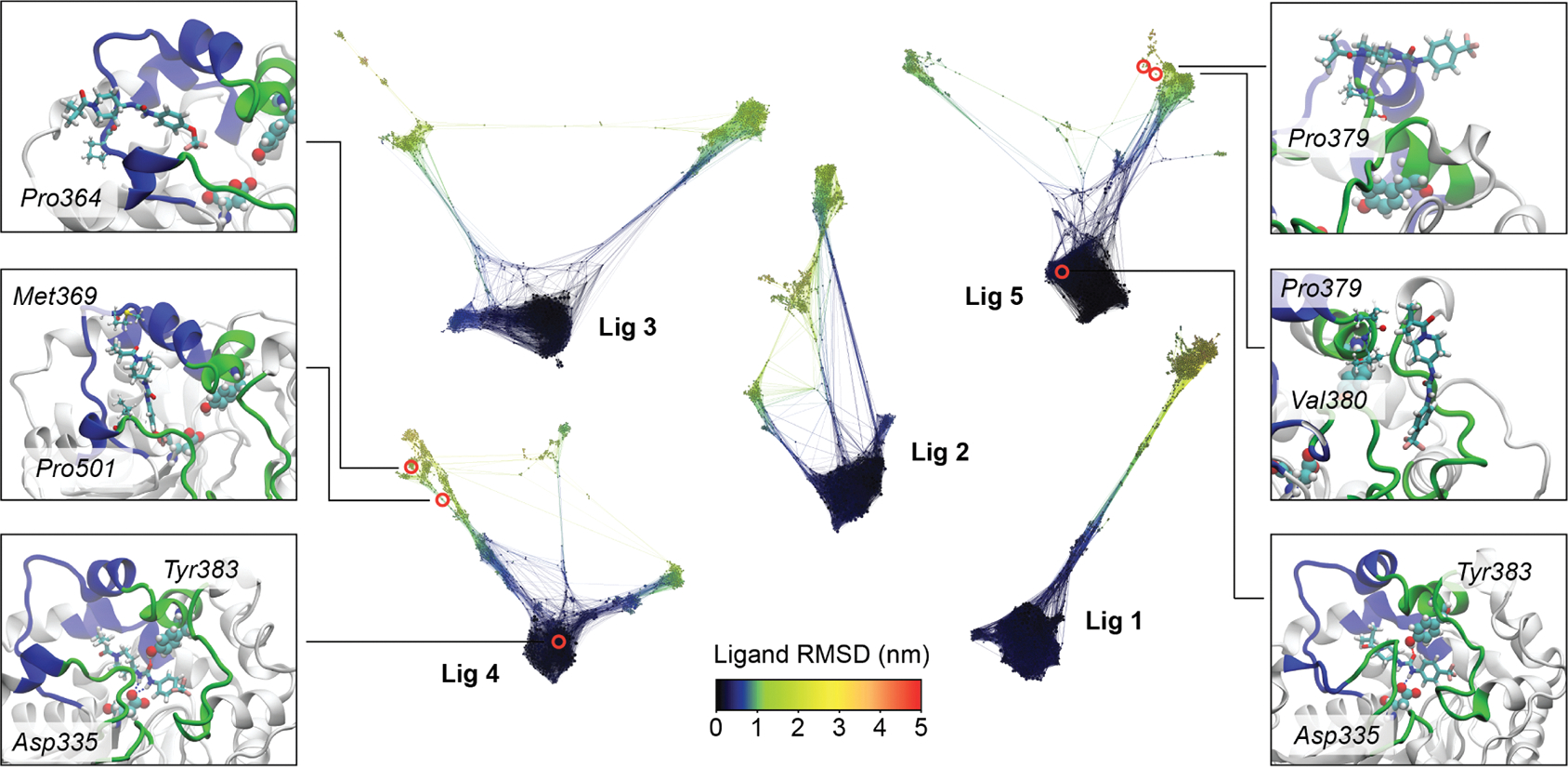
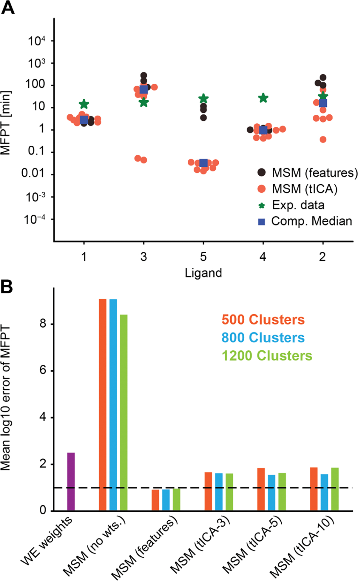
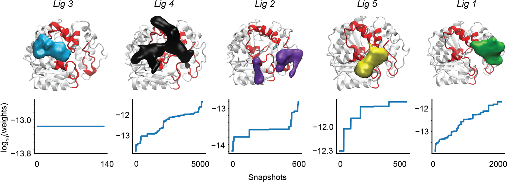
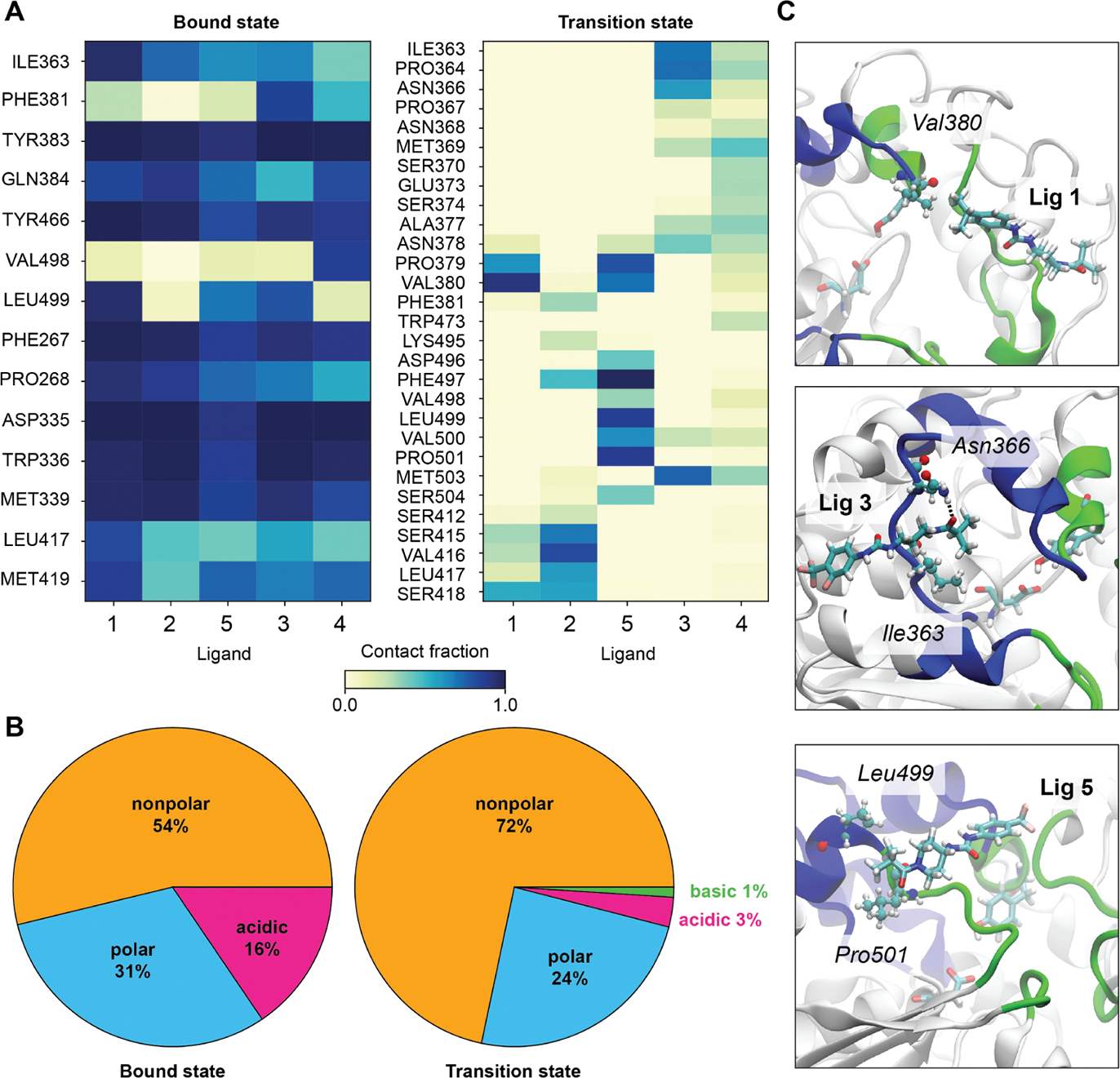
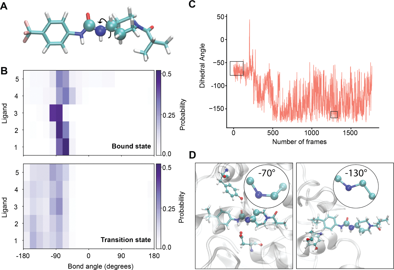
For many drug targets, it has been shown that the kinetics of drug binding (e.g., on rate and off rate) is more predictive of drug efficacy than thermodynamic quantities alone. This motivates the development of predictive computational models that can be used to optimize compounds on the basis of their kinetics. The structural details underpinning these computational models are found not only in the bound state but also in the short-lived ligand binding transition states. Although transition states cannot be directly observed experimentally due to their extremely short lifetimes, recent successes have demonstrated that modeling the ligand binding transition state is possible with the help of enhanced sampling molecular dynamics methods. Previously, we generated unbinding paths for an inhibitor of soluble epoxide hydrolase (sEH) with a residence time of 11 min. Here, we computationally modeled unbinding events with the weighted ensemble method REVO (resampling of ensembles by variation optimization) for five additional inhibitors of sEH with residence times ranging from 14.25 to 31.75 min, with average prediction accuracy within an order of magnitude. The unbinding ensembles are analyzed in detail, focusing on features of the ligand binding transition state ensembles (TSEs). We find that ligands with similar bound poses can show significant differences in their ligand binding TSEs, in terms of their spatial distribution and protein-ligand interactions. However, we also find similarities across the TSEs when examining more general features such as ligand degrees of freedom. Together these findings show significant challenges for rational, kinetics-based drug design.

Figure 1.

sEH protein and its inhibitors: (A) 2D representation of sEH inhibitors; (B) the combined epoxide-phosphatase domain: the binding region is highlighted in red; (C) the Ligand2 bound sEH protein with the two most interacting residues in the bound state.

Figure 2.

(A) The scheme of extracting TSE from weighted ensemble MD data with MSMs. (B) Visual representation of the interatomic ligand-binding site distance features for a ligand, which are later used to cluster the simulation data. The yellow spheres are ligand–atom representations, and blue spheres are the backbone atoms of the residues constituting the binding site. (C) All ligand conformations from a particular microstate after clustering all the frames based on distance features. (D) Microstates and their connectivity from a transition probability matrix. (E) CSN of ligand 4, with ligand RMSD being the scale of color. The densely populated bound state is shown in dark blue, and the sparsely connected unbound states are shown in yellow/red.

Figure 3.

CSNs of ligand unbinding from sEH in the scale of the ligand RMSD. The networks are arranged and oriented according to pathway specificity. Three frames from the most probable unbinding pathways are highlighted for ligand 4 (cavity specificity: left) and ligand 5 (cavity specificity: right). The states corresponding to those frames are highlighted in the CSNs. In each panel, the ligands are shown in licorice while the amino acid residues within 2.5 Å of the ligands are depicted in CPK representation, with the binding site Asp335 and Tyr383 highlighted in vdW representation.

Figure 4.

(A) Computational prediction of MFPTs for each ligand with all MSMs is plotted together as a swarmplot. The full feature space MSMs (black circles) perform better compared to tICA-based MSMs (red circles). The experimental data (green asterices) are plotted along with the medians of all computational estimates (blue boxes). The ligands are ordered in the ascending order of experimental residence times. (B) Comparison of the root mean squared log-10 error plotted for various MSMs (red, blue, and green) and direct estimates from WE weights (violet). The MSM using the full feature set has the lowest RMS log-10 error, while the unweighted MSM has the highest RMS log-10 error. The horizontal line marks an average error of 1 order of magnitude.

Figure 5.

(Top row) Density plots of the ligand unbinding TSEs: different ligands are plotted in different colors. The two binding site residues Asp335 and Tyr383 are shown in the licorice representation, while the overall binding region is highlighted by a red color. Each surface is plotted in VMD using the same density cutoff (“isovalue”) of 0.05. (Bottom row) Weights of conformations used to build the TS ensembles are plotted on a log-scale for each ligand. The horizontal axis shows the number of independent snapshots in the TSE. The vertical axis shows the log₁₀ of the weight of that snapshot.

Figure 6.

Protein–ligand interactions in the ligand unbinding TS ensembles of sEH: (A) Heatmap of interaction probabilities in bound and TSE for the ligands; colorbar denotes the measure of probability. The ligands which unbind through the right side of the cavity (ligands 1, 2, and 5) are placed first in the horizontal axis, followed by the ligands unbinding through the left side of the cavity (ligands 3 and 4). (B) Pie chart describing the category of protein–ligand interactions based on the type of the amino acids, averaged over all the ligands. (C) Representations of a few of the most probable interactions in TS ensembles for ligands 1, 3, and 5.

Figure 7.

(A) The atoms corresponding to the rotatable bond with the largest difference between the bound ensemble and the TSE are shown in the van der Waals representation, with other atoms in licorice representation. (B) Probability distributions of this angle are shown for each ligand in both the bound ensemble (top) and TSE (bottom). (C) The value of this dihedral angle is shown over the course of the most probable unbinding trajectory for ligand 1. The black boxes indicate the frames corresponding to the bound (left) and TS (right) ensembles. (D) Representative snapshots of the bound (left) and TS (right) ensembles, showing the dihedral angle in the insets.

References

1. Greer J; Erickson JW; Baldwin JJ; Varney MD Application of the Three-Dimensional Structures of Protein Target Molecules in Structure-Based Drug Design. J. Med. Chem. 1994, 37, 1035–1054. - PubMed
1. Rutenber EE; Stroud RM Binding of the anticancer drug ZD1694 to E. coli thymidylate synthase: Assessing specificity and affinity. Structure 1996, 4, 1317–1324. - PubMed
1. Wlodawer A; Vondrasek J Inhibitors of HIV-1 protease: A major success of structure-assisted drug design. Annu. Rev. Biophys. Biomol. Struct. 1998, 27, 249–284. - PubMed
1. Clark DE What has computer-aided molecular design ever done for drug discovery? Expert Opin. Drug Discovery 2006, 1, 103–110. - PubMed
1. Veldkamp CT; Ziarek JJ; Peterson FC; Chen Y; Volkman BF Targeting SDF-1/CXCL12 with a Ligand That Prevents Activation of CXCR4 through Structure-Based Drug Design. J. Am. Chem. Soc. 2010, 132, 7242–7243. - PMC - PubMed
Publication types