Multiple Concurrent Predictions Inform Prediction Error in the Human Auditory Pathway

Abstract

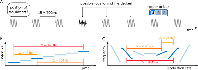
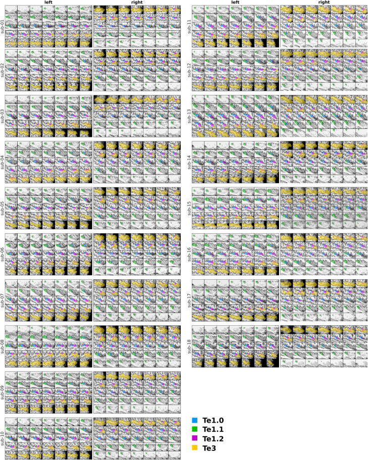
The key assumption of the predictive coding framework is that internal representations are used to generate predictions on how the sensory input will look like in the immediate future. These predictions are tested against the actual input by the so-called prediction error units, which encode the residuals of the predictions. What happens to prediction errors, however, if predictions drawn by different stages of the sensory hierarchy contradict each other? To answer this question, we conducted two fMRI experiments while female and male human participants listened to sequences of sounds: pure tones in the first experiment and frequency-modulated sweeps in the second experiment. In both experiments, we used repetition to induce predictions based on stimulus statistics (stats-informed predictions) and abstract rules disclosed in the task instructions to induce an orthogonal set of (task-informed) predictions. We tested three alternative scenarios: neural responses in the auditory sensory pathway encode prediction error with respect to (1) the stats-informed predictions, (2) the task-informed predictions, or (3) a combination of both. Results showed that neural populations in all recorded regions (bilateral inferior colliculus, medial geniculate body, and primary and secondary auditory cortices) encode prediction error with respect to a combination of the two orthogonal sets of predictions. The findings suggest that predictive coding exploits the non-linear architecture of the auditory pathway for the transmission of predictions. Such non-linear transmission of predictions might be crucial for the predictive coding of complex auditory signals like speech.Significance Statement Sensory systems exploit our subjective expectations to make sense of an overwhelming influx of sensory signals. It is still unclear how expectations at each stage of the processing pipeline are used to predict the representations at the other stages. The current view is that this transmission is hierarchical and linear. Here we measured fMRI responses in auditory cortex, sensory thalamus, and midbrain while we induced two sets of mutually inconsistent expectations on the sensory input, each putatively encoded at a different stage. We show that responses at all stages are concurrently shaped by both sets of expectations. The results challenge the hypothesis that expectations are transmitted linearly and provide for a normative explanation of the non-linear physiology of the corticofugal sensory system.

Keywords: auditory midbrain; auditory pathway; cortico-thalamic interactions; predictive coding; sensory processing; sensory thalamus.

Figure 1.

Experimental design. A, Example of a trial. Each trial consisted of a sequence of seven repetitions of one standard (gray) and a single instance of a deviant (black). The deviant could occur in positions 4, 5, or 6 of the sequence. Participants reported, in each trial, the position of the deviant immediately after they identified it. Within a sequence, stimuli were separated by 700 ms ISIs. B, The three pure tones used in the pure tone experiment are displayed in dark blue. Trials were characterized by the absolute difference between the frequency of the standard and the deviant $\mathrm{\Delta }$. C, The three FM-sweeps used in the FM-sweep experiment are displayed in dark blue. Trials were characterized by the absolute difference between the modulation rate of the standard and the deviant $\mathrm{\Delta }$. The stimuli schematically shown in light blue in panels B and C were not used in the experiments and are plotted here only to contextualize the used stimuli within a family characterized by a continuously varying property (frequency in B and modulation rate in C).

Figure 2.

Anatomical location of the subcortical ROIs in each participant. Each panel plots the location of each ROI projected from MNI to the structural space of the participant using the coregistration inverse transform.

Figure 3.

Anatomical location of the cortical ROIs in each participant (pure tone experiment). Each panel plots the location of each ROI projected from MNI to the structural space of the participant using the coregistration inverse transform.

Figure 4.

Anatomical location of the cortical ROIs in each participant (FM-sweeps experiment). Each panel plots the location of each ROI projected from MNI to the structural space of the participant using the coregistration inverse transform.

Figure 5.

Schematics of t.eps models used for Bayesian model comparison. Each panel plots a possible linear combination of the regressors used in each of the three models for each of the nine trial types (three deviant positions $\times$ three values of $\mathrm{\Delta }$) of the experiments. Plots in panel A show the stats model, and in panel B, the task model, and in C, the combined model. Each colored line corresponds to one $\mathrm{\Delta }$ value (red corresponds to the largest delta, yellow to the lowest). The apparent delay between colored lines is a visualization device: there was no such delay in the model. Note that the relative height of the first standard (in comparison to the deviant) and the relative weight that $\mathrm{\Delta }$ has in the responses to the deviants are free parameters of the model.

Figure 6.

Bayesian model comparison in IC and MGB. A, Experiment 1 (pure tones). Maps detailing which model best explained the responses to pure tones in each of the voxels of the IC and MGB ROIs. Colors indicate the model with the highest posterior density at each voxel of the IC and MGB ROIs. Blue voxels are best explained by the stats model, green voxels by the task model, purple voxels by the combined model, and yellow voxels by the control model, taken here as baseline. B, Distributions (kernel-density estimations) of the $K$ factors comparing the performance of each of the first three models again the control model across voxels of the IC and MGB rois. C, The same as in A, but for Experiment 2 (FM-sweeps). D, The same as in B, but for Experiment 2 (FM-sweeps).

Figure 7.

Bayesian model comparison in the primary and secondary subdivisions of the MGB. Distributions (kernel-density estimations) of the $K$ factors comparing the performance of each of the first three models again the control model across voxels of the MGB subdivisions from Mihai et al. (2019) for the pure tone and FM-sweep stimuli. Distributions are qualitatively comparable in the primary MGB and the rest of the nucleus (secondary MBG) for both experiments.

Figure 8.

Prevalence of each model in AC for pure tones. A, Map detailing which model best explains the responses to pure tones in each of the voxels of the AC. Colors indicate the model with the highest posterior density at each voxel. Blue voxels are best explained by the stats model, green voxels by the task model, and purple voxels by the combined model. B, Distributions (kernel-density estimations) of the posterior densities of each model across voxels of each of the cortical fields for the pure tone stimuli.

Figure 9.

Prevalence of each model in AC for FM-sweeps. A, Map detailing which model best explains the responses to FM-sweeps in each of the voxels of the AC. Colors indicate the model with the highest posterior density at each voxel. Blue voxels are best explained by the stats model, green voxels by the task model, and purple voxels by the combined model. B, Distributions (kernel-density estimations) of the posterior densities of each model across voxels of each of the cortical fields for the FM-sweep stimuli.

Figure 10.

Prevalence of each model in each cortical field. Bars show the prevalence of each of the models across cortical fields for the pure tone A and FM-sweep B data. Blue bars correspond to voxels that are best explained by the stats model, green bars to voxels best explained by the task model, and purple bars to voxels best explained by the combined model.

References

1. Altmann CF, Gaese BH (2014) Representation of frequency-modulated sounds in the human brain. Hear Res 307:74–85. 10.1016/j.heares.2013.07.018 - DOI - PubMed
1. Avants BB, Tustison NJ, Song G, Cook PA, Klein A, Gee JC (2011) A reproducible evaluation of ANTs similarity metric performance in brain image registration. NeuroImage 54:2033–2044. 10.1016/j.neuroimage.2010.09.025 - DOI - PMC - PubMed
1. Baron-Cohen S, Wheelwright S, Hill J, Raste Y, Plumb I (2001) The “Reading the mind in the eyes” test revised version: a study with normal adults, and adults with Asperger syndrome or high-functioning autism. J Child Psychol Psychiatry 42:241–251. 10.1111/jcpp.2001.42.issue-2 - DOI - PubMed
1. Bekinschtein TA, Dehaene S, Rohaut B, Tadel F, Cohen L, Naccache L (2009) Neural signature of the conscious processing of auditory regularities. Proc Natl Acad Sci U S A 106:1672–1677. 10.1073/pnas.0809667106 - DOI - PMC - PubMed
1. Brainard DH (1997) The psychophysics toolbox. Spat Vis 10:433–436. 10.1163/156856897X00357 - DOI - PubMed
Publication types
LinkOut - more resources