. 2023 Nov 20;3(11):100636.
doi: 10.1016/j.crmeth.2023.100636. Epub 2023 Nov 13.

Instant processing of large-scale image data with FACT, a real-time cell segmentation and tracking algorithm

Affiliations

Instant processing of large-scale image data with FACT, a real-time cell segmentation and tracking algorithm

Ting-Chun Chou et al. Cell Rep Methods. .

Abstract

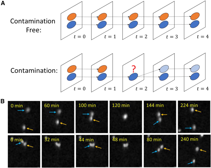
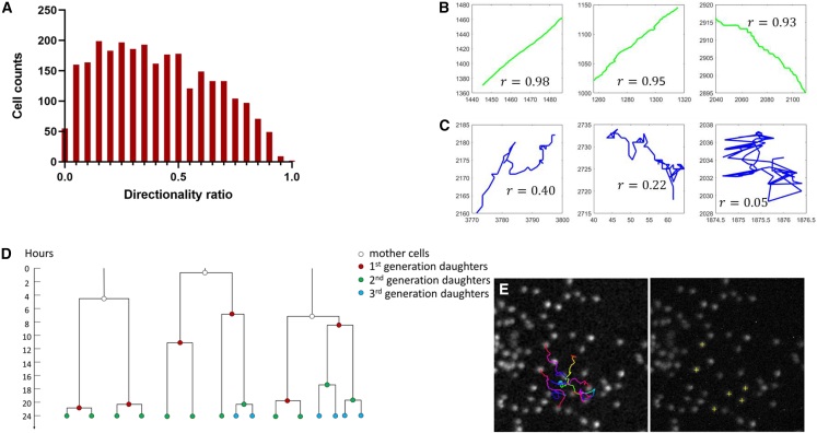
Quantifying cellular characteristics from a large heterogeneous population is essential to identify rare, disease-driving cells. A recent development in the combination of high-throughput screening microscopy with single-cell profiling provides an unprecedented opportunity to decipher disease-driving phenotypes. Accurately and instantly processing large amounts of image data, however, remains a technical challenge when an analysis output is required minutes after data acquisition. Here, we present fast and accurate real-time cell tracking (FACT). FACT can segment ∼20,000 cells in an average of 2.5 s (1.9-93.5 times faster than the state of the art). It can export quantifiable features minutes after data acquisition (independent of the number of acquired image frames) with an average of 90%-96% precision. We apply FACT to identify directionally migrating glioblastoma cells with 96% precision and irregular cell lineages from a 24 h movie with an average F1 score of 0.91.

Keywords: CP: Imaging; cell tracking correction; high-throughput imaging; lineage tracking; live-cell imaging; machine-learning-based cell segmentation; real-time cell tracking.


Conflict of interest statement

Declaration of interests The authors declare no competing interests.

Figures

None
Graphical abstract
Figure 1
Figure 1
Ground-truth-assisted trainable Weka segmentation (GTWeka) pipeline The original TWS pipeline is highlighted in blue. (A) Image features, generated by applying all default image filters on an input image. (B) Data annotation (or labeling). Manual assignment of pixels to three classes: nucleus (blue), background (green), and edge (red). (C) Training data, a combination of annotated pixels and their corresponding values from image features. (D) Random forest classifier, which is trained with the input training data. (E) We then use the well-trained model to perform the semantic segmentation. Connected component analysis is applied to generate the instance segmentation from the semantic segmentation. If needed, users can improve the segmentation performance by adding more annotations and re-training the classifier (steps A–D) until no further improvement is observed. The processes from (A)–(E) take ∼30–60 min. Our GTWeka (highlighted in red) improves the segmentation speed via GPU-based operation and key feature selection and increases the segmentation accuracy by incorporating ground-truth reference data (F), which only requires 30–60 min of preparation. The reference data are used to optimize the random forest classifier. Reference data are generated from a number of cropped regions of the original input image and labeled as individual nuclei and background.
Figure 2
Figure 2
Benchmarking of cell segmentation methods (GTWeka, TWS, ilastik, StarDist, CellSeg, and Cellpose) (A) Cell segmentation using different Weka-based segmentation methods with different cell image datasets (MCF10A, GBM, and HeLa). Images from top to bottom: raw image, images processed by GTWeka_all features, GTWeka_selected features (3 features), TWS, ilastik_all features, and ilastik_selected features (3 features by the ilastik_filter method). (B) Comparison of performance (average F1 score at IoU = 0.5 or 0.7) and processing time (s) of all the methods mentioned in (A). Fast processing, as much as possible to the degree of seconds, is crucial for applications of identifying rare cells out of a large population; see Figure S4. (C) Cell segmentation using GTWeka and other deep-learning-based methods (StarDist, CellSeg, and Cellpose) with different cell image datasets (MCF10A, GBM, and HeLa). Images from top to bottom: raw image, images processed by GTWeka_selected features (3 features), StarDist, CellSeg, and Cellpose. (D) Comparison of performance (average F1 score at IoU = 0.5 or 0.7) and processing time (s) of all the methods mentioned in (C).
Figure 3
Figure 3
Cell merging and demerging (A) Graphical illustration of two complete tracks (top) and incomplete tracks (bottom). For the contaminated case, two cells merge at frame t=2, giving rise to (1) a false division at frame t=3 and (2) an incomplete track of the orange cell that ends at frame t=1. (B) Two examples of the merging-demerging problem shown in the raw image data of GBM cells. Top: two cells (blue and orange arrows) merge for over 30 min and then deviate. A snapshot at time “120 min” shows the merging event. Bottom: two cells (blue and orange arrows) merge twice at times “32 min” and “48 min.” This is caused by both complicated cell behaviors as well as false segmentation.
Figure 4
Figure 4
Cell track correction (A) Graphic illustration of cell track correction. (Top) Step 1: examine if a division is valid. We see that a merging at t=2 causes a cell track (orange) to disappear at location xdisappear and a demerging at t=3 causes a division at location xdivide. The false cell division is detected when the event is next to an incomplete track within a pre-defined (Euclidean) distance (Δx between xdisappear and xdivide) and within a pre-defined time window (time difference, Δt, between the merging and demerging events). (Middle) Step 2: remove the link of a false division. Compared to step 1, the frames with changes are highlighted in yellow. We disconnect the link (green) from t=2 to t=3 (in step 1), as this daughter cell (green) is closer to xdisappear than the other daughter cell (blue). The link removal generates an incomplete track (green) from t=3 to t=4. (Bottom) Step 3: close the gap between the incomplete tracks. Compared to step 2, the frames with changes are highlighted in yellow. The two incomplete tracks (orange and green) are to be connected. There is a gap between them, which refers to the disappeared cell at t=2. We then construct a fake cell (gray) at this frame at any location of xgenerate between xdisappear and xdivide. We update the reconstructed cell to the subsequent frames t=3,4. At t=4, we obtain two complete tracks. (B) Merging-demerging caused a false division (top). The tracks are corrected with our cell track correction method (bottom). (C) Merging-demerging caused three false divisions (top) (merging happened at “76 min,” “120 min,” and “264 min”), and tracks were corrected with our cell track correction method (bottom).
Figure 5
Figure 5
Application of FACT to identify abnormal cancer cells (A–C) GBM cell tracking. (A) Distribution of directionality ratio (r) over 2,724 cells. Over all cells, we looked for the ones giving a ratio r > 0.90. (B) Example trajectories of cells with directional walk; directionality ratio (r) is indicated per cell. (C) Example trajectories of cells without directional walk; directionality ratio (r) is indicated per cell. (D and E) Cell lineage tracking of MCF10A cells. (D) Topology of lineages from 3 groups, “tree-3-div” (left), “tree-4-div” (middle), and “tree-5-div” (right). In each plot, time is represented as the vertical axis, going from 0 to 24 h. Daughter cells generated in different generations are color-coded. Videos of these cases are included in Video S1. (E) Migratory trajectories of the lineage of interest (tree-5-div) (left image), and the final coordinates of the cells (yellow cross, right image).
Figure 6
Figure 6
FACT tracking steps (A) Nuclear-mask images as input for tracking. The input images are the pixel-wise dot product of raw and GTWeka segmented images. (B) Transforming each input It into a mixture of Gaussian models (GMs) Gt, where each cell i is considered as one Gaussian git. The properties of a Gaussian (i.e., mean, variance) can describe a cell’s location and shape. And a Gaussian distribution itself denotes a cell’s intensity. Frame-to-frame linking per cell is performed by “finding nearest neighbors of Gaussians between adjacent frames” if we say a cell's position in one frame is the nearest neighboring location to its position in the next frame. The nearest neighbors are searched in multidimensions, including changes of location, shape, and intensity. The algorithm behind is Bayesian inference, a probabilistic model that calculates expected changes (e.g., location, intensity, shape) of all cells (per frame) over time. Similar cells are linked over time. Division can be followed by examining if one Gaussian is splittable. (C) Forwarding GMs gives initial tracking outcomes, which might be prone to contamination. The outcomes are saved in XML files. Here, we visualize them as a table. Cells that are tracked at each frame generate “complete tracks.” Cells that are missed for at least one frame generate “incomplete tracks.” (D) Correction of tracks that are contaminated. The correction goes sequentially as follows: (1) looking for false divisions, with the information of detected divisions and incomplete tracks. (2) Breaking the mother-daughter link if a false division is confirmed. The breakup also generates new incomplete tracks. (3) Updating the incomplete tracks with new ones. (4) Bridging the incomplete tracks as one complete track (a way of closing gaps). A gap refers to the spatial and temporal distance between two (or more) track segments; meanwhile, these track segments are parts of one same cell track.
Figure 7
Figure 7
Comparing FACT tracking to other popular tracking approaches such as linear assignment problem (LAP) When cells are prone to move toward each other, often causing overlapping, FACT gives higher precision and F1 score regarding cell division estimation. Details of cell track correction used by LAP and our FACT method are summarized in this figure.

Similar articles

Cited by

References

    1. Stegmaier J., Amat F., Lemon W.C., McDole K., Wan Y., Teodoro G., Mikut R., Keller P.J. Real-Time Three-Dimensional Cell Segmentation in Large-Scale Microscopy Data of Developing Embryos. Dev. Cell. 2016;36:225–240. doi: 10.1016/j.devcel.2015.12.028. - DOI - PubMed
    1. Amat F., Lemon W., Mossing D.P., McDole K., Wan Y., Branson K., Myers E.W., Keller P.J. Fast, accurate reconstruction of cell lineages from large-scale fluorescence microscopy data. Nat. Methods. 2014;11:951–958. doi: 10.1038/nmeth.3036. - DOI - PubMed
    1. You L., Su P.-R., Betjes M., Rad R.G., Chou T.-C., Beerens C., van Oosten E., Leufkens F., Gasecka P., Muraro M., et al. Linking the genotypes and phenotypes of cancer cells in heterogenous populations via real-time optical tagging and image analysis. Nat. Biomed. Eng. 2022;6:667–675. doi: 10.1038/s41551-022-00853-x. - DOI - PubMed
    1. Pantazis P., Supatto W. Advances in whole-embryo imaging: a quantitative transition is underway. Nat. Rev. Mol. Cell Biol. 2014;15:327–339. doi: 10.1038/nrm3786. - DOI - PubMed
    1. Masuzzo P., Van Troys M., Ampe C., Martens L. Taking Aim at Moving Targets in Computational Cell Migration. Trends Cell Biol. 2016;26:88–110. doi: 10.1016/j.tcb.2015.09.003. - DOI - PubMed

Publication types

LinkOut - more resources