

doi: 10.1118/1.595967.
Phase and sensitivity of receiver coils in magnetic resonance imaging
- PMID: 3796476
- PMCID: PMC2396267
- DOI: 10.1118/1.595967
Item in Clipboard
Phase and sensitivity of receiver coils in magnetic resonance imaging
Med Phys.
1986 Nov-Dec.
Abstract
Receiver coil response is a major cause of nonuniformities in magnetic resonance images. The spatial dependence of the sensitivity and phase of single-saddle receiver coils has been investigated quantitatively by calculating the H1 field and comparing the results with measurements of a uniform phantom. Agreement between the measurements and calculations is excellent. A method is developed which corrects for both the nonuniform sensitivity and the phase shifts introduced by receiver coils.
Figures
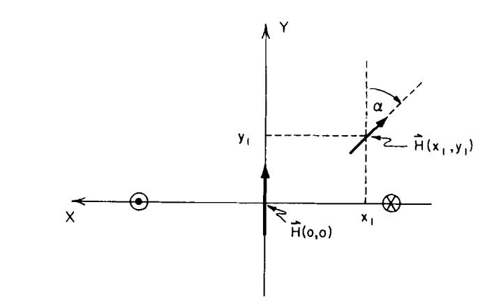
Two H1 vectors in the vector field produced by a current through a single-saddle coil. The straight elements of the coil puncture the plane at the positions marked by the circles. The direction of the current flow is shown.
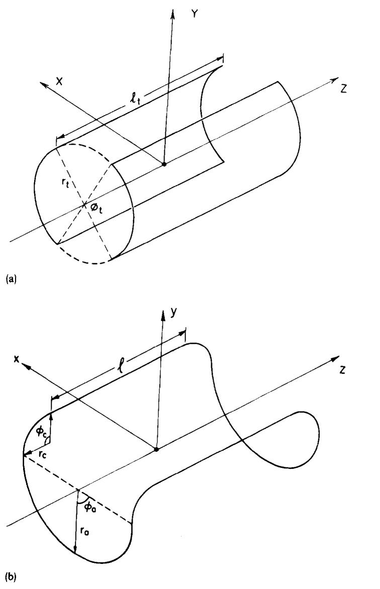
Coil configuration used as the example for this paper. (a) The geometry of the double-saddle transmitter coil. (b) A schematic of a single-saddle receiver coil.
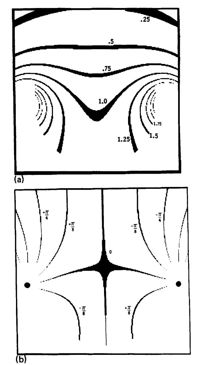
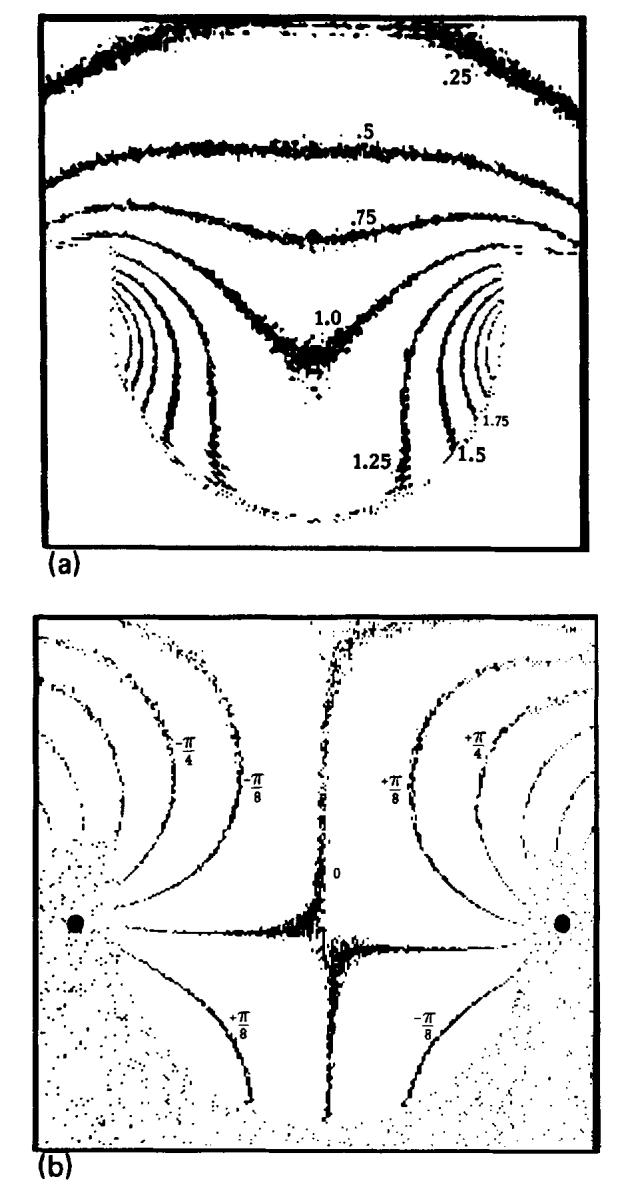
Two contour plots which characterize the H1 field of the receiver coil in the z = 0 plane, as shown in Fig. 2(b). (a) A contour plot of |H1(x, y)|. The contour lines are separated by units of 0.25 of the central amplitude which is set to 1.0. The contour widths are 0.5% of the contour value. (b) A contour plot of the phase of the H1 field, α(x, y). The plots have been multiplied by a mask outlining the phantom used in the experiment.
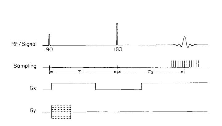
Pulse sequence used to collect data for phase images.
Measured coil sensitivity and phase. (a) A contour plot of the measured relative magnitudes of image vectors r(x, y) for a uniform phantom. (b) An isophase contour plot of the measured phase φ(x, y).
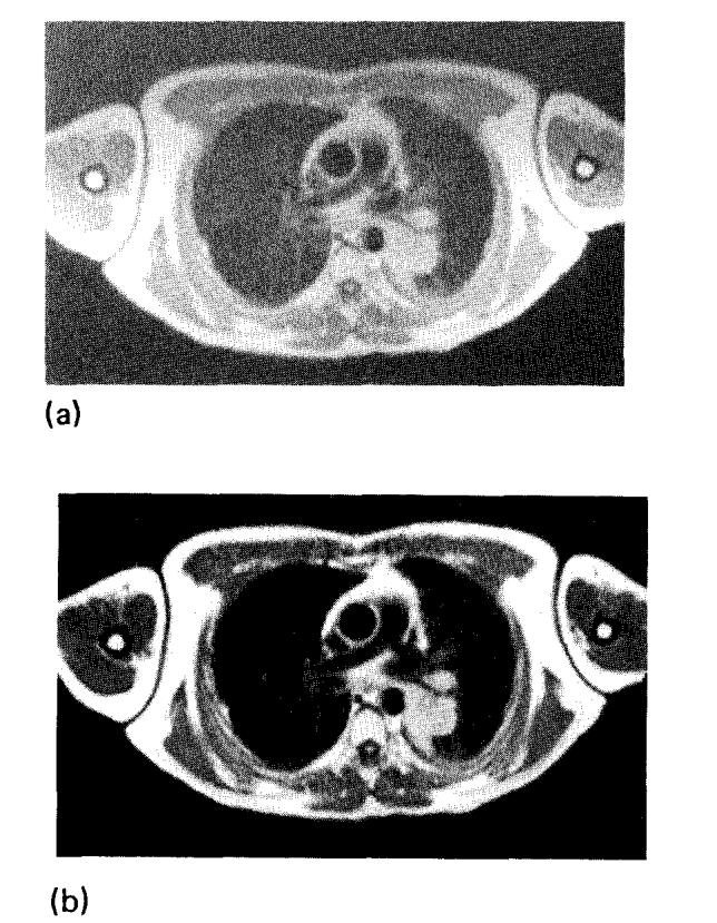
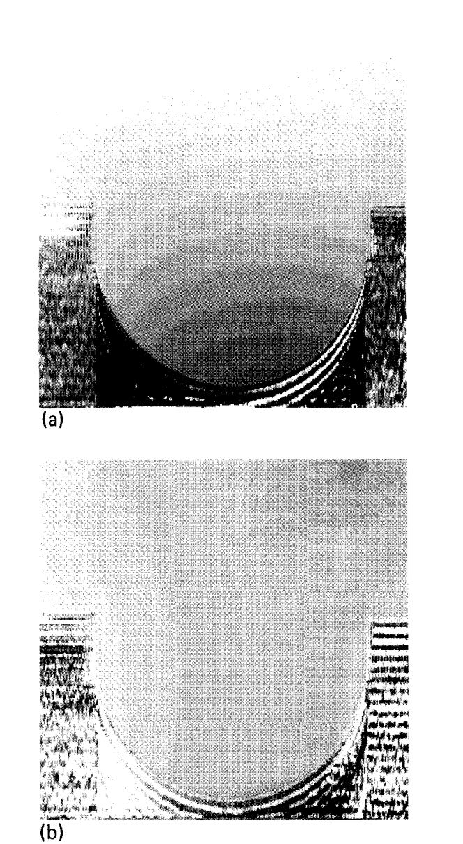
(a) SE image (TR = 1200, TE = 30) of a transverse plane through the mediastinum. (b) The same image after correction for the coil sensitivity. The window was set to the same value for both images.
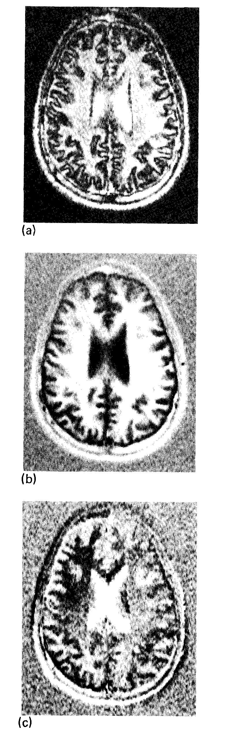
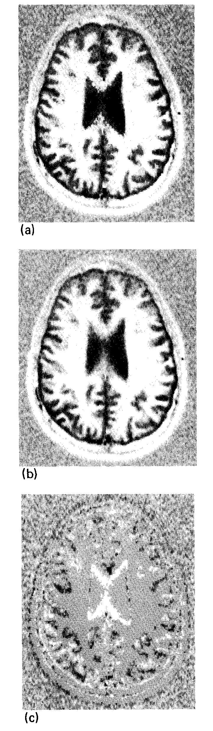
Transverse images of a 1-cm slice through the head obtained with an ISE sequence (TR = 2000 ms, TI = 240 ms, TE = 30 ms). (a) Using magnitude reconstruction, phase information is lost and regions of long TI, such as CSF and GM, have inverted, positive signal intensity. (b) The “real” component of the complex image. This image is phase sensitive. (c) The “imaginary” image is the projection of the image vectors onto the axis orthogonal to that in (b). The window for (b) is 20 times the background root-mean-square deviation, the window for (a) and (c) is 10 times the background rms deviation of (b).
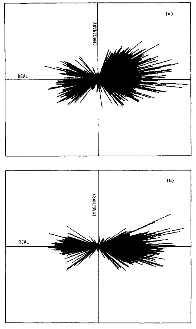
(a) Plot of image pixels in the complex plane. The pixels shown are from the left-half of the head in Fig. 7 and exclude background. (b) The same pixels as in (a), after subtracting the measured phase errors.
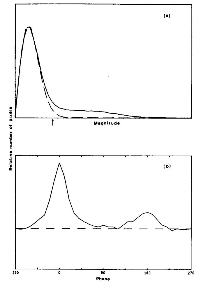
Histograms of the magnitude and phase of image pixels from the image shown in Fig. 7, after subtraction of the estimated phase error. (a) The distribution of the pixel magnitudes is the solid curve P(m); the dashed line shows a Rayleigh distribution R(m). The arrow marks the m value where R(m)/P(m) = 0.5. (b) The distribution of phase angles found in the image.
Same image as shown in Fig. 7 with an attempt to display the full magnitude of the image vectors with the correct sign. (a) A simple algorithm which uses the sign of the real part of the image vector after phase correction to determine the sign of the displayed pixel. Note the increased low-signal noise, jagged boundaries, and anaomalous pixels. (b) The phase sensitive image after the image processing described in the text. (c) The residual signal remaining in the imaginary image after this processing. The window for (a) and (b) is the same as in Fig. 7(b); the window for (c) is the same as in Fig. 7(c).
Magnetic field inhomogeneity images constructed from phase differences. Each step in the gray scale represents ∼4 ppm. (a) Before initial first-order corrections. (b) After first-order corrections in the vertical direction.
Similar articles
-
Solenoid surface coils in magnetic resonance imaging.AJR Am J Roentgenol. 1986 Feb;146(2):409-12. doi: 10.2214/ajr.146.2.409. AJR Am J Roentgenol. 1986. PMID: 3484592
-
In vivo method for correcting transmit/receive nonuniformities with phased array coils.Magn Reson Med. 2005 Mar;53(3):666-74. doi: 10.1002/mrm.20377. Magn Reson Med. 2005. PMID: 15723397
-
MR spectroscopy using multi-ring surface coils.Magn Reson Med. 1999 Oct;42(4):655-64. doi: 10.1002/(sici)1522-2594(199910)42:4<655::aid-mrm6>3.0.co;2-d. Magn Reson Med. 1999. PMID: 10502753
-
Radiofrequency coils for magnetic resonance applications: theory, design, and evaluation.Crit Rev Biomed Eng. 2014;42(2):109-35. doi: 10.1615/critrevbiomedeng.2014011482. Crit Rev Biomed Eng. 2014. PMID: 25403875 Review.
-
Theory and application of array coils in MR spectroscopy.NMR Biomed. 1997 Dec;10(8):394-410. doi: 10.1002/(sici)1099-1492(199712)10:8<394::aid-nbm494>3.0.co;2-0. NMR Biomed. 1997. PMID: 9542737 Review.
Cited by
-
A new bias field correction method combining N3 and FCM for improved segmentation of breast density on MRI.Med Phys. 2011 Jan;38(1):5-14. doi: 10.1118/1.3519869. Med Phys. 2011. PMID: 21361169 Free PMC article.
-
A phased array coil for human cardiac imaging.Magn Reson Med. 1995 Jul;34(1):92-8. doi: 10.1002/mrm.1910340114. Magn Reson Med. 1995. PMID: 7674903 Free PMC article.
-
Recommendations of Choice of Head Coil and Prescan Normalize Filter Depend on Region of Interest and Task.Front Neurosci. 2021 Oct 29;15:735290. doi: 10.3389/fnins.2021.735290. eCollection 2021. Front Neurosci. 2021. PMID: 34776844 Free PMC article.
-
Phase-sensitive inversion recovery for detecting myocardial infarction using gadolinium-delayed hyperenhancement.Magn Reson Med. 2002 Feb;47(2):372-83. doi: 10.1002/mrm.10051. Magn Reson Med. 2002. PMID: 11810682 Free PMC article.
-
Medial femur T2 Z-scores predict the probability of knee structural worsening over 4-8 years: Data from the osteoarthritis initiative.J Magn Reson Imaging. 2017 Oct;46(4):1128-1136. doi: 10.1002/jmri.25662. Epub 2017 Feb 16. J Magn Reson Imaging. 2017. PMID: 28206712 Free PMC article.
References
-
- Bydder GM, Butsen PC, Harman RR, Gilderdale DJ, Young IR. J. Comput. Assist. Tomogr. 1985;9:413. - PubMed
-
- Glover GH, Hayes CE, Pelc NJ, Edelstein WA, Mueller OM, Hart HR, Hardy CJ, O’Donnell M, Barber WD. J. Magn. Reson. 1985;64:255.
-
- Leroy-Willig A, Darrasse L, Taquin J, Sauzadi M. Magn. Reson. Med. 1985;2:20. - PubMed
-
- Hinshaw WS, Gauss RC. Distributed phase rf coil. European Patent Application, Publ. No. 0047065. 1981.
-
- Hayes CE, Edelstein WA, Schenck JF, Mueller OW, Eash M. 1985; presented at the Soc. Magn. Reson. Med., Fourth Annual Meeting; London.
Publication types
MeSH terms
Grants and funding
LinkOut - more resources
Full Text Sources
Other Literature Sources
