Machine learning for microbiologists

Abstract

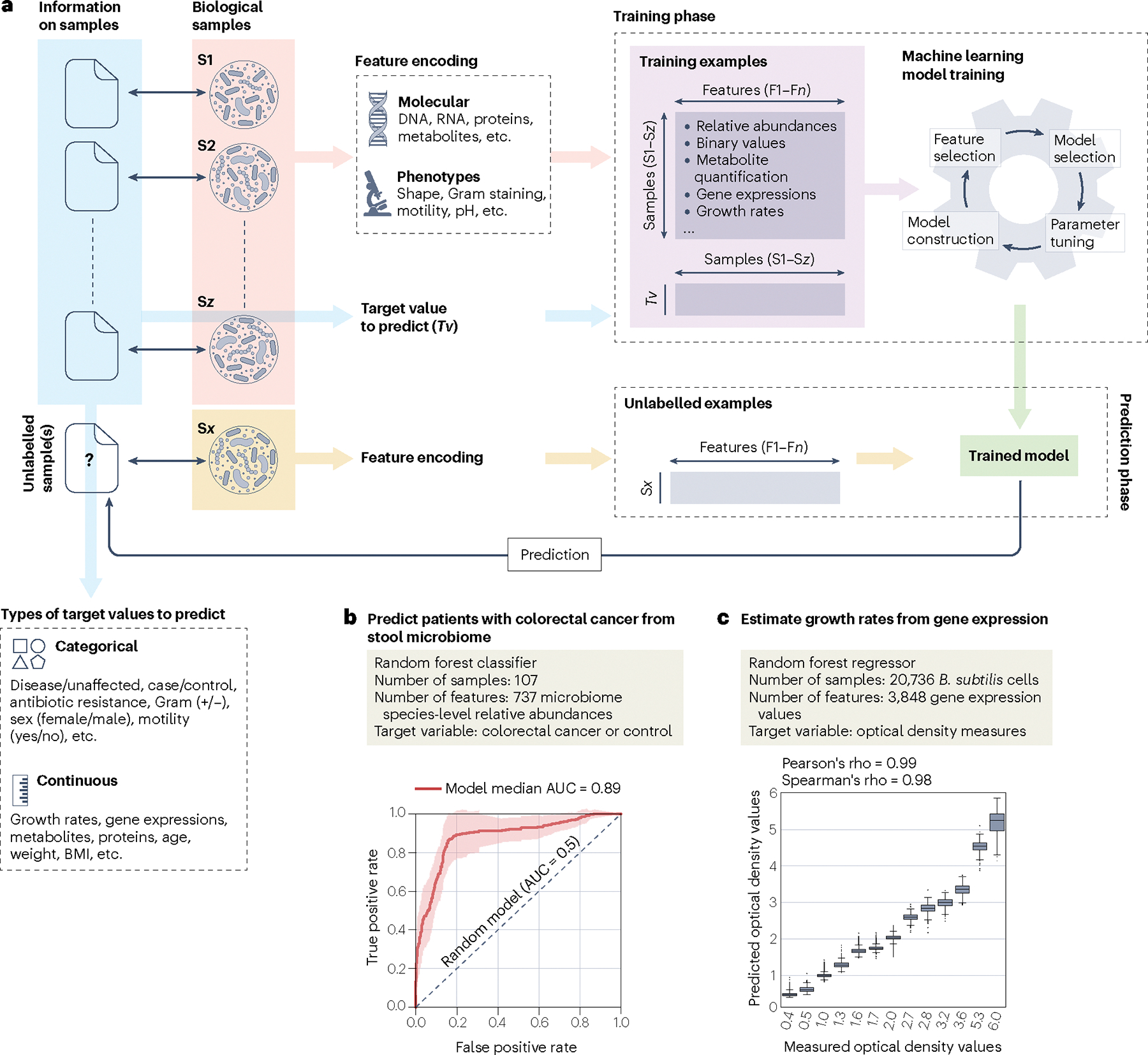
Machine learning is increasingly important in microbiology where it is used for tasks such as predicting antibiotic resistance and associating human microbiome features with complex host diseases. The applications in microbiology are quickly expanding and the machine learning tools frequently used in basic and clinical research range from classification and regression to clustering and dimensionality reduction. In this Review, we examine the main machine learning concepts, tasks and applications that are relevant for experimental and clinical microbiologists. We provide the minimal toolbox for a microbiologist to be able to understand, interpret and use machine learning in their experimental and translational activities.

Fig. 1 |. General workflow and examples for machine learning applications in microbiology.

a, High-level workflow of supervised machine learning describing different types of molecular (DNA, RNA, proteins and so on) and phenotypic (morphology, motility, pH and so on) characteristics derived from biological samples (pink background) that form the set of features (indicated as F1–Fn), and target values generated from potential other information (blue background) associated with the biological samples (indicated with double-headed black arrows). The ‘Training phase’ details the input data (for example, relative abundance, metabolite quantification, gene expression and so on; violet background) and the steps that will produce the trained model, which include model selection, adjustment of the parameters, construction of the model and feature selection. The same set of features used for training the model but derived from new unseen and unlabelled biological samples (yellow background) are the input for the trained model (‘Prediction phase’) to predict the unknown corresponding outcome variable (‘?’). b, Application of supervised learning, using 737 species-level relative abundance values as input features to classify 107 stool microbiome samples into control versus colorectal cancer categories (original data from ref. and available in ref. 120). This example uses the random forest classification algorithm and shows the median model’s performance (bold red line). For comparison, the dashed black line shows the performances of a random model. c, Application of supervised learning to estimate Bacillus subtilis growth rates (measured as optical density) from 3,848 gene expression values from more than 20,000 B. subtilis cells as input features. The example uses the random forest regression algorithm and reports the distributions of the predicted optical density values for each of the measured values. AUC, area under the curve; BMI, body mass index.

Fig. 2 |. Practical examples of unsupervised learning tasks.

a, k-Means is a clustering algorithm that requires an a priori number of clusters (k) into which samples are grouped. In the example, k-means with k = 2 was applied on Jaccard distances calculated using the protein content of 3,598 genomes collected by Méheust et al. from four published data sets^– and visualized using principal component analysis (PCA). This data set includes 22,977 protein clusters representing 4,449,296 sequences from 2,321 candidate phyla radiation (CPR) genomes, 1,198 non-CPR bacterial genomes and 79 archaeal genomes. PCA is used for visualization and points are coloured according to cluster assignment. The two clusters, Cluster 1 and Cluster 2, separate according to the assigned taxonomy, with Cluster 1 containing most of the CPR genomes falling within a single cluster. Bar plot shows the fraction of genomes assigned to each cluster (top right). b, Heatmap showing the presence (yellow) and absence (black) profiles of the protein clusters (columns) across the genomes (rows). The genomes were sorted using agglomerative hierarchical clustering applied on Jaccard pairwise distances and calculated using the protein content of the genomes. Hierarchical clustering defines clusters by ‘cutting’ the hierarchical tree at a certain height. In the example, two clusters can be defined, and also in this case Cluster 1 contains most of the CPR genomes. Bar plot shows the fraction of original labels assigned to each of the 3,598 genomes separated into the two clusters as defined by the hierarchical tree (as in panel a for the clusters defined by k-means). c, PCA is a dimensionality reduction technique used to visualize high-dimensional data into a lower-dimensional space. Points represent each of the individual genomes with taxonomic kingdoms overlaid on the plot for visual exploration. Bar plot shows the first six principal components that explain most of the variance across the genomes according to their protein content (top right). d, Each component of the PCA can explain a fraction of the variance present in the data. The first two components, for instance, explain 29% of the variance, and the first principal component alone already permits partial separation of taxonomic divisions of origin of the protein clusters.

Fig. 3 |. Training and testing strategies for supervised machine learning model evaluation.

a,b, Supervised machine learning training (lighter boxes) and testing (bold boxes) strategies for when a single data set is available using splitting and re-sampling. Splitting one single data set into two subsets (usually with 80% and 20% of the samples, respectively) and using the larger one for model training and the smaller for model testing (panel a). k-Fold cross-validation iterates the previous splitting strategy k times (usually k = 5 or 10). It is also possible to repeat the k-fold cross-validation multiple times with random choices of the samples belonging to the folds. This strategy improves the validation power of the left-out same data set as it is less dependent on the choice of the samples in the testing set (panel b). c,d, Multi-data sets training and testing strategies using cross-data set or leave-one-data set-out (LODO) approaches. A cross-data set approach exploits one data set for training the model and the other independent data set for testing it. This is a better estimation of the generalization power of the model compared with single data set evaluations as it directly tests the performances of a different data set with potentially unavoidable differences (panel c). When more than two data sets are available, the LODO approach exploits n – 1 data sets for the training phase and uses the left-out data set for testing, repeating for all data sets. It combines the improved generalizability of the model when trained on distinct data sets with potentially different underlying differences with the comprehensive evaluation performed on multiple left-out data sets (panel d).

Fig. 4 |. Supervised machine learning evaluation methods in a real-data example.

The diagnosis potential of colorectal cancer using only stool microbiome features with a supervised machine learning approach. a, We applied biased and unbiased training and testing strategies to detect colorectal cancer in three publicly available data sets using faecal quantitative species-level relative abundances^,,. Boxplots show area under the receiver operating characteristic (ROC) curve (AUC-ROC) values obtained via training a random forest model on true labels (colorectal cancer versus control; top panel) and randomized labels (no biological signal; bottom panel). For ‘original labels’, different training and testing strategies can lead to differences in the estimated classifiers’ performances, especially when considering the model generalizability to other independent cohorts. For ‘randomized labels’, an overfitted classifier can perform better in cross-validation but will not generalize well on other independent data sets and can completely invalidate an experiment by fitting the noise of a single cohort. We show the results of model evaluation using single data sets and multi-data set training and testing strategies (as in Fig. 3). Cross-data set evaluation of unbiased classifiers achieves lower AUC-ROCs than cross-validation, which is expected given the unavoidable differences between data sets, but is a more reliable evaluation of how the model would perform on new data. To show the effects of overfitting on model performance, we ran the same analysis but pre-selected the ten species with the lowest significant unadjusted P value (P < 0.05, Wilcoxon rank-sum test). As expected, the biased classifier that would perform very well on the training set is outperformed by the unbiased one in the evaluation on test sets. Importantly, the biased classifier still performs well in cross-validation, but this is the result of overfitting as the result is also obtained when the labels are randomly assigned (and so no AUC-ROC significantly above 0.5 is possible). b, Cross-prediction matrix showing AUC-ROC mean values obtained via training a random forest model to detect colorectal cancer in four publicly available data sets using faecal quantitative species-level relative abundances^,,,. The matrix encompasses both single data set cross-validation and multi-data set training and testing strategies to evaluate the model’s performance. Among the described approaches, the leave-one-data set-out (LODO) AUC-ROCs should be regarded as the best possible estimations of the performance the model should achieve on new data.

References

1. Bishop CM Pattern recognition and machine learning (Springer, 2006).
1. Hastie T, Tibshirani R & Friedman J The Elements of Statistical Learning: Data Mining, Inference, and Prediction 2nd edn (Springer Science & Business Media, 2009).
1. James G, Witten D, Hastie T & Tibshirani R An Introduction to Statistical Learning: with Applications in R (Springer Science & Business Media, 2013).
1. Murphy KP Probabilistic Machine Learning: Advanced Topics (MIT Press, 2022).
1. Goodswen SJ et al. Machine learning and applications in microbiology. FEMS Microbiol. Rev. 45, fuab015 (2021). - PMC - PubMed
LinkOut - more resources