Fast multiple-trait genome-wide association analysis for correlated longitudinal measurements

Abstract

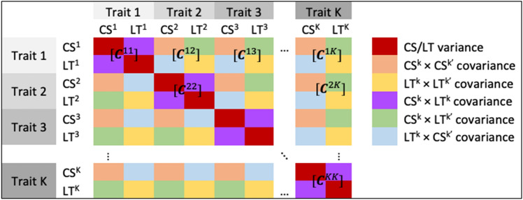
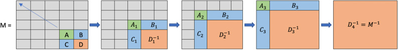
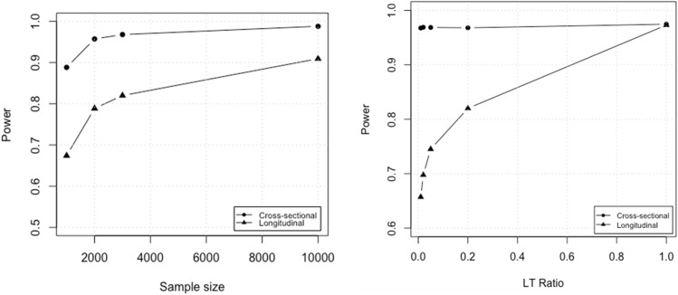
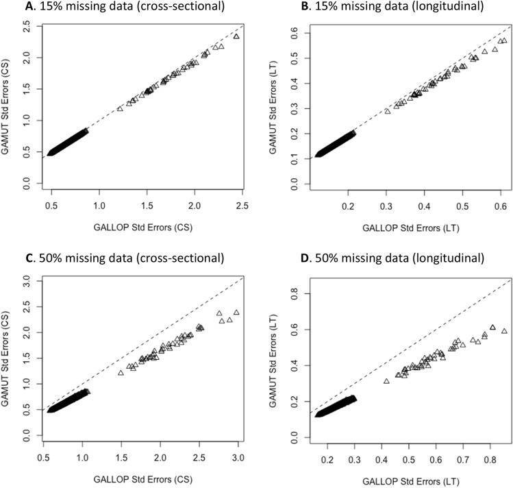
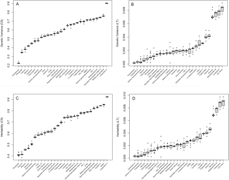
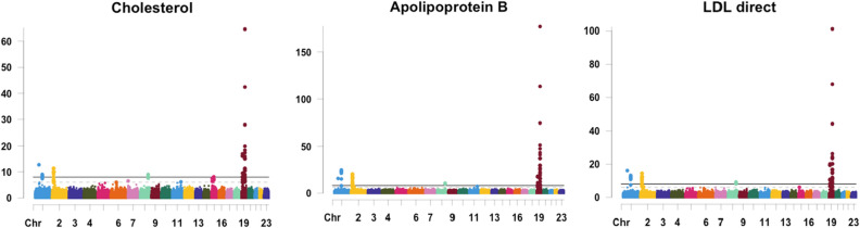
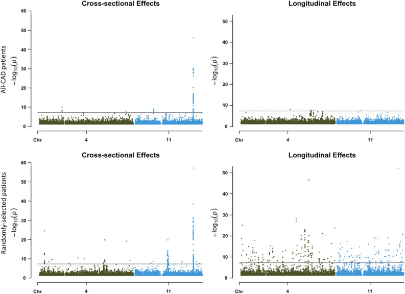
Large-scale longitudinal biobank data can be leveraged to identify genetic variation contributing to human diseases progression and traits trajectories. While methods for genome-wide association studies (GWAS) of multiple correlated traits have been proposed, an efficient multiple-trait approach to model longitudinal phenotypes is not currently available. We developed GAMUT, a genome-wide association approach for multiple longitudinal traits. GAMUT employs a mixed-effects model to fit longitudinal outcomes where a fast algorithm for inversion by recursive partitioning of the random effects submatrix is introduced. To evaluate performance of the algorithms introduced and assess their statistical power and type I error, stochastic simulation was conducted. Consistent with our expectation, power was greater for cross-sectional (CS) than longitudinal (LT) effects, particularly with a diminishing LT/CS ratio. With a minimum minor allele count of 3 within genotype by time categories, observed type I error was roughly equal to theoretical genome-wide significance. Additionally, 28 blood-based biomarkers measured at 2 time points on participants of the UK Biobank were used to compare GAMUT against single-trait standard and longitudinal GWAS (including rate of change). Across all biomarkers, we observed 539 (CS) and 248 (LT) significant independent variants for the GAMUT method, and 513 (CS) and 30 (LT) for single-trait longitudinal GWAS, respectively. Only 37 variants were identified by modeling rates of change using standard GWAS.

Figure 1

Inverse of the genetic variance and covariance matrix among $K$ traits. Each ${\mathit{C}}^{k{k}^{\prime }}$ submatrix corresponds to the ${(k{k}^{\prime })}^{\mathit{th}}$ 2 × 2 block of the pairwise covariance between cross-sectional and longitudinal effects of traits $k$ and $k^{\prime }$.

Figure 2

Schematic for inversion by recursive partitioning where the inverse of the lower-right corner of 4 submatrices is integrated in the next round as the inverse of the greater D (or D₁), etc. Note that in each round, e.g. $\rho ,$ ${\mathit{D}}_{\rho }^{-1}$ replaced ${\mathit{D}}_{\rho }$ because the ${\mathit{D}}_{\mathit{\rho }}$ submatrix itself was not needed in round $\rho +1$.

Figure 3

Statistical power of identifying causal variants using GAMUT. Powers are shown for 4 sample sizes in the left panel and 5 longitudinal to cross-sectional ratios in the right panel. Powers shown are calculated as averages of 3 phenotypes over 100 replicates per scenario. Power of detecting causal longitudinal effects was smaller than those of cross-sectional effects, particularly for relatively smaller longitudinal effects. Sample size simulations of the left panel were based on 1:5 LT to CS, ratios which resulted in a consistently lower longitudinal curve.

Figure 4

Standard errors of multiple-trait, GAMUT versus single-trait, GALLOP for two scenarios, one with 15% missing records (A,B) and another with 50% missing records (C,D) in 1 out of 3 simulated phenotypes. GAMUT consistently reduced standard errors of genetic variants scanned for the phenotype with missing records. Dotted line is the slope of GAMUT Std Errors on equivalent values.

Figure 5

Cross-sectional and longitudinal statistical power estimates in simulated scenarios with 0, 15, and 50% of individuals missing. In the single-trait approach, missing individuals directly impacted sample size and significantly reduced power of the phenotype with missing data, relative to the multiple-trait approach which utilized the correlation between traits to compensate for the reduction in sample size. In the simulation, the sample size with no missing records was 3000 and the LT to CS ratio was set to 1:5.

Figure 6

Actual time for direct sparse inversion and inversion by recursive partitioning of Z’R^–1Z + G^-–1. For 20 traits, runtime for direct sparse invasion was extrapolated to 130 min vs. 2.2 min of actual runtime for inversion by recursive partitioning. Direct inversion was highly exponential versus recursive inversion that was nearly linear in the number of traits.

Figure 7

(A) Total system setup and association times for the single- and multiple-trait runs, modeled up to 12 traits in the largest cluster. Multiple-trait analyses were far more run-time efficient vs. single-trait, despite following an exponential curve. (B) extrapolated time up to 20 traits in analysis; multiple-trait cost exceeded that of single-trait after 16 traits.

Figure 8

(A) Polygenic cross-sectional (CS) variances estimated between traits in a pairwise fashion where Lipoprotein A produced the highest variance and Testosterone showed the least genetic variance. (B) Longitudinal variances (LT) variances estimated alongside the CS variances using AI-REML. LDL direct, Cholesterol, Apolipoprotein B, and Glucose had the greatest variances and Testosterone had near-zero longitudinal variance. (C) Cross-sectional polygenic heritability estimates. (D) Longitudinal polygenic heritability estimates. CS polygenic variance and heritability estimates were generally much greater than those for LT, indicating that more cross-sectional associations are expected to be identified. Further, CS polygenic variance and heritability estimates were relatively more consistent compared with those for LT.

Figure 9

Polygenic and residual covariance and correlation between Testosterone and all other biomarker traits, sorted by covariance. (A1,A2) Cross sectional variance components estimates, showing SHBG (circled points on the scatter plot) as the trait with the strongest correlation. SHBG is a protein made by the liver and binds itself to sex hormones in both sexes. (B1,B2) Longitudinal variance component estimates, showing SHBG among the top correlated traits, indicating parallel progression at the genetic level between the two traits. (C1,C2) show the residual variance component estimates with high SHBG correlation that is not as strong as the genetic correlations.

Figure 10

Cross-sectional genetic (A), longitudinal genetic (B), and residual (C) correlation for a cluster of biomarker traits. Genetic and residual correlations were positive and strong among LDL direct, Apolipoprotein B and Cholesterol. In the correlation plots above, thin lines reflect strong correlation and thick lines toward oval and circular shapes indicate weaker correlations toward 0.

Figure 11

Cross-sectional p-values of all biomarker traits (1532 variants before LD clumping). Significant variants from conventional rate of change GWAS (138 variants before LD clumping) indicated with red triangles. Only the most significant cross-sectional variants were captured by conventional GWAS on rates of change.

Figure 12

Manhattan plots of cross-sectional variants for 3 genetically correlated traits analyzed jointly using multiple-trait longitudinal GWAS.

Figure 13

Manhattan plots of cross-sectional and longitudinal variants for primary care triglycerides with 3 to 35 repeated measures on CAD-diagnosed patients. Multiple genome-wide significant hits were identified for the two effect types.

Figure 14

Manhattan plots of cross-sectional and longitudinal variants on chromosomes 4 and 11 for primary care triglycerides with 3 to 35 repeated measures on CAD-diagnosed patients on the top 2 panels vs. a randomly selected sample on the bottom panels. The homogeneous sample with CAD did not show as much inflation as with the random sample.

References

1. Sikorska K, Lesaffre E, Groenen PJF, Rivadeneira F, Eilers PHC. Genome-wide analysis of large-scale longitudinal outcomes using penalization -GALLOP algorithm. Sci. Rep. 2018;8(1):6815. doi: 10.1038/s41598-018-24578-7. - DOI - PMC - PubMed
1. Jiang L, Zheng Z, Fang H, Yang J. A generalized linear mixed model association tool for biobank-scale data. Nat. Genet. 2021;53(11):1616–1621. doi: 10.1038/s41588-021-00954-4. - DOI - PubMed
1. Kang HM, Zaitlen NA, Wade CM, Kirby A, Heckerman D, Daly MJ, Eskin E. Efficient control of population structure in model organism association mapping. Genetics. 2008;178:1709–1723. doi: 10.1534/genetics.107.080101. - DOI - PMC - PubMed
1. Zhou X, Stephens M. Genome-wide efficient mixed model analysis for association studies. Nat. Genet. 2012;44:821–824. doi: 10.1038/ng.2310. - DOI - PMC - PubMed
1. Zhou W, Zhao Z, Nielsen JB, Fritsche LG, LeFaive J, Taliun SAG, Bi W, et al. Scalable generalized linear mixed model for region-based association tests in large biobanks and cohorts. Nat. Genet. 2020;52:634–639. doi: 10.1038/s41588-020-0621-6. - DOI - PMC - PubMed