Robust mapping of spatiotemporal trajectories and cell-cell interactions in healthy and diseased tissues

Abstract

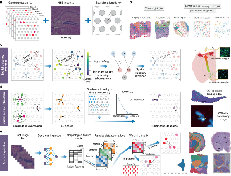
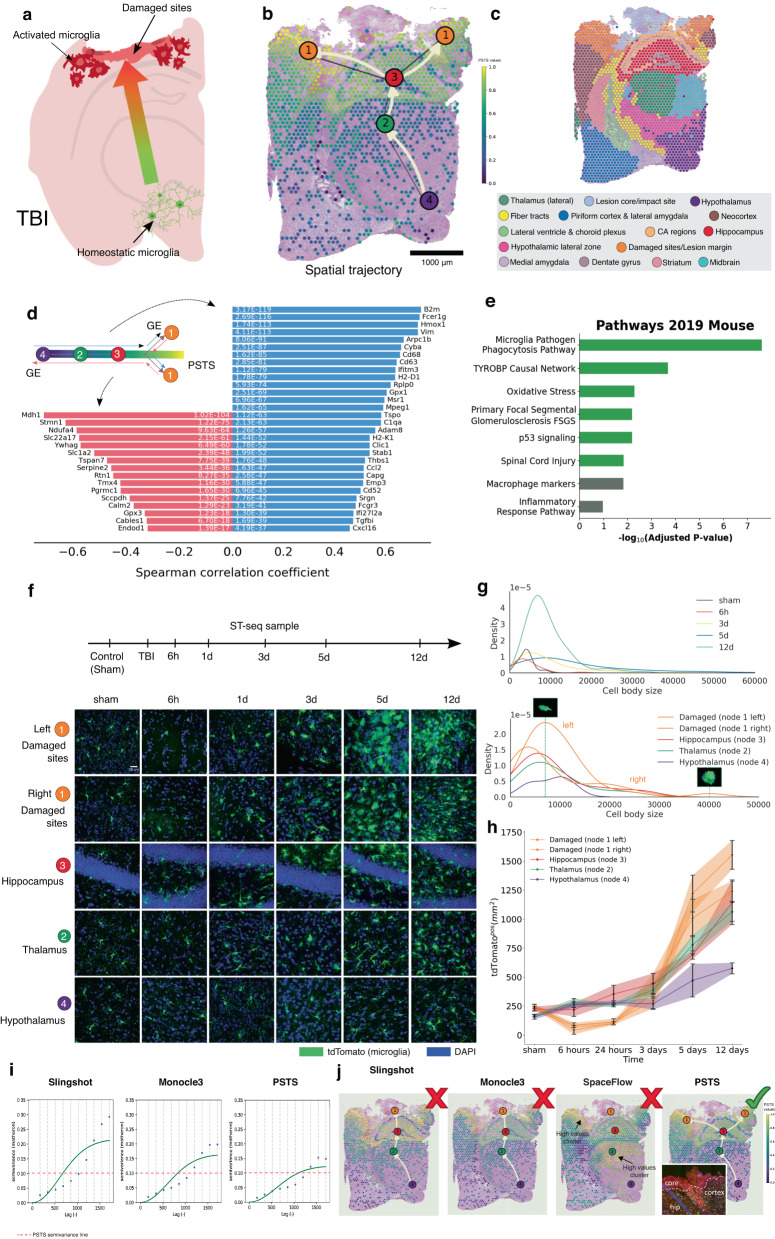
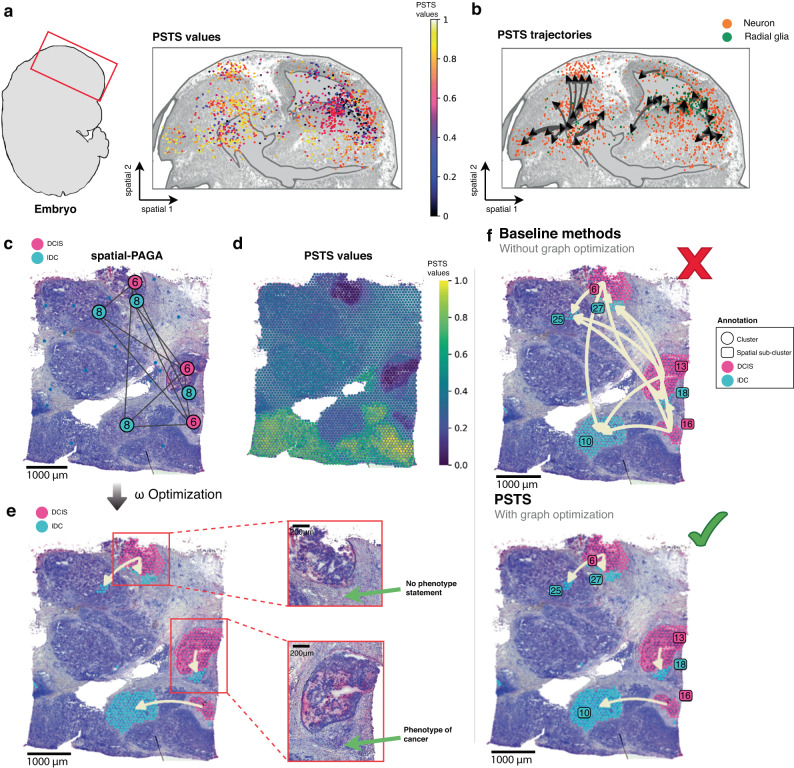
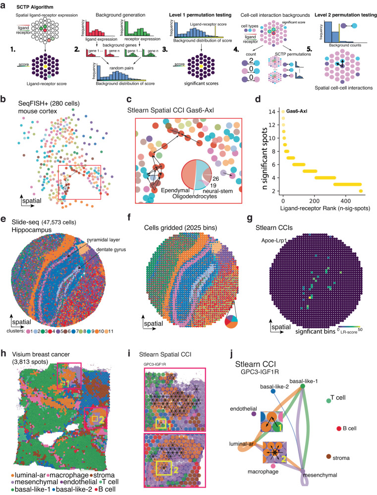
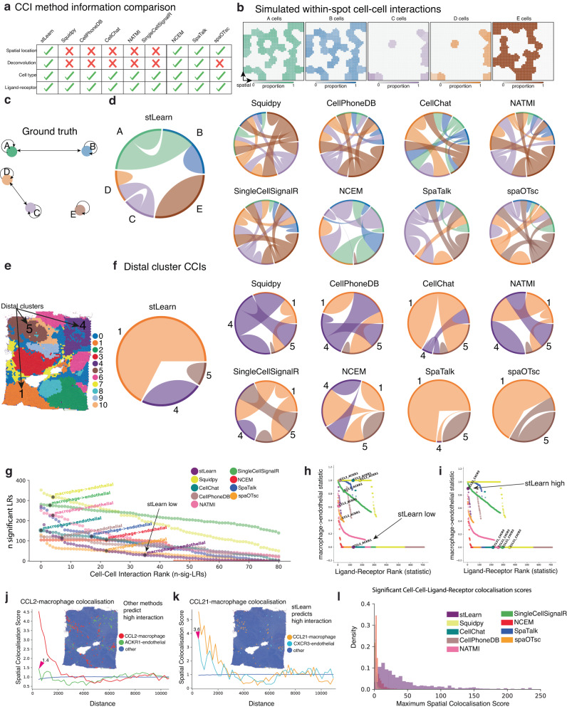
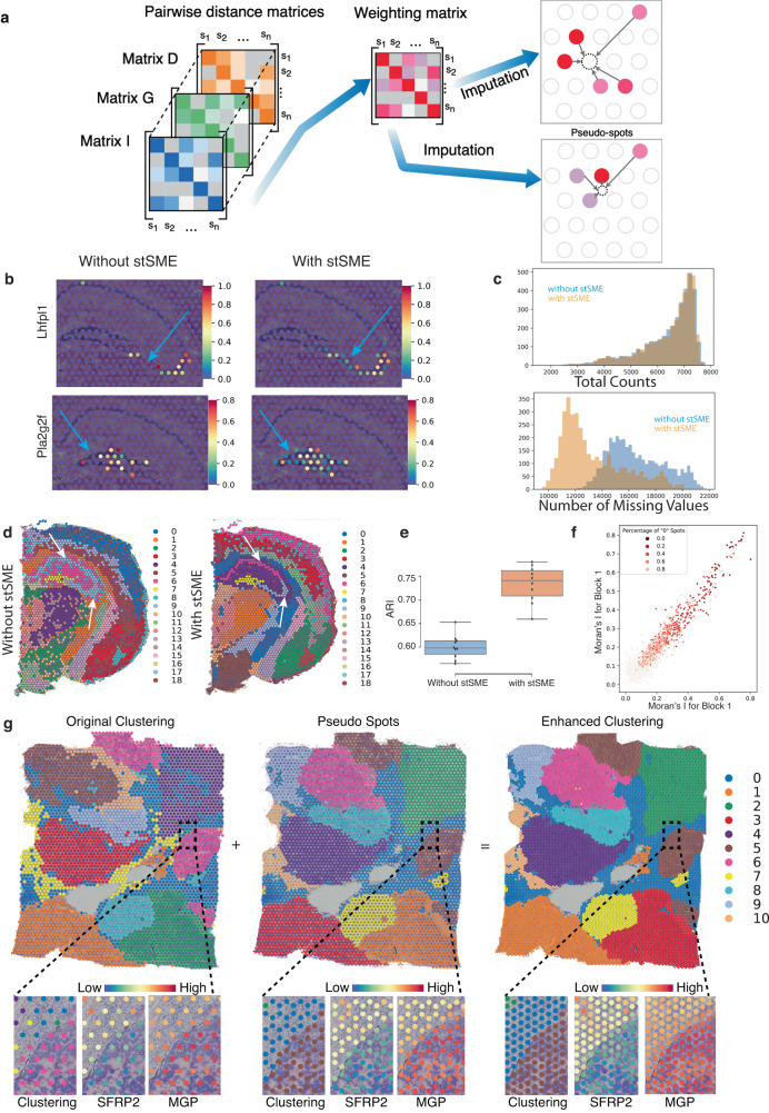
Spatial transcriptomics (ST) technologies generate multiple data types from biological samples, namely gene expression, physical distance between data points, and/or tissue morphology. Here we developed three computational-statistical algorithms that integrate all three data types to advance understanding of cellular processes. First, we present a spatial graph-based method, pseudo-time-space (PSTS), to model and uncover relationships between transcriptional states of cells across tissues undergoing dynamic change (e.g. neurodevelopment, brain injury and/or microglia activation, and cancer progression). We further developed a spatially-constrained two-level permutation (SCTP) test to study cell-cell interaction, finding highly interactive tissue regions across thousands of ligand-receptor pairs with markedly reduced false discovery rates. Finally, we present a spatial graph-based imputation method with neural network (stSME), to correct for technical noise/dropout and increase ST data coverage. Together, the algorithms that we developed, implemented in the comprehensive and fast stLearn software, allow for robust interrogation of biological processes within healthy and diseased tissues.

Fig. 1. Spatial analysis algorithms implemented in stLearn.

a Schematic diagram showing the three spatial data types that can be integrated by stLearn: gene expression (G), imaging (I) and spatial distance (D). b stLearn can be applied to a range of spatial technologies, with or without tissue imaging information (using f(G, I, D) or f(G, D) functions). c Spatial trajectory analysis to infer biological processes within an undissociated tissue. Pseudo-space-time distance (PSTD) values are calculated based on gene expression and physical distance. Spatial distance is calculated between the centroid coordinates of clusters U and V with sub-clusters (u₁, u₂) and (v₁, v₂, v₃). PSTD values are used to construct a rooted, directed graph (arborescence), the topology of which can be optimised by a minimum spanning tree to infer the trajectory. This approach to trajectory analysis was validated in a mouse model of traumatic brain injury. d Spatially-constrained two-level permutation (SCTP) analysis for cell–cell interaction (CCI) between (straight arrows) and within (looped arrows) spatial spots. SCTP uses ligand and receptor co-expression information among neighbouring spots, and cell type diversity (gradient blue spots; darker colour indicates more cell types per spot) to compute ligand-receptor (LR) scores. SCTP finds hotspots (purple) within a given tissue, where LR interactions between cell types are more likely to occur compared to a null distribution of random non-interacting gene-gene pairs. Predicted interactions were confirmed by RNA single molecule imaging. e Overview of within-tissue imputation and clustering by stSME, which corrects for technical noise (dropouts) in gene expression values by using imaging data (via a neural network model - matrix I), and spots that are both physically near and have similar gene expression profiles (distance matrices D and G, respectively). stSME can also predict gene expression in tissue regions for which there is no experimental data (pseudo-spots). stSME clustering performance was validated against an established anatomical reference mouse brain (spatial brain data, top far right), or expert pathologist annotation (breast cancer data, bottom far right).

Fig. 2. Pseudo-time-space (PSTS) trajectory analysis and validation in a mouse model of traumatic brain injury (TBI).

a Schematic showing the cortical impact site and microglia activation. b Spatio-temporal trajectory of microglial activation at 3 days post-TBI, as predicted by our PSTS algorithm, running from the hypothalamus (node 4), through the thalamus (node 2) and hippocampus (node 3) and then the cortical penumbra regions adjacent to the lesion core (nodes 1). Colour-coded pseudo-time-space values (ranging from 0 to 1) reflect microglia-related gene expression changes through the tissue space. c Clustering results for TBI Visium ST data (n = 2442 spots). d Transition genes positively (blue) or negatively (red) correlated with the predicted trajectory for microglia activation (extracted by Spearman correlation test of pseudo-time-space values; adjusted p-value < 0.05 and correlation coefficient >0.3 or <−0.3). e Enrichment analysis of upregulated transition genes revealing significant pathways related to microglia activation, inflammation and neural injury. f Experimental validation of the spatio-temporal trajectory for microglia (green) activation following TBI; cell nuclei are shown in blue. Imaging was performed across five different brain regions of interest (ROIs; from one brain per time point), equivalent to the trajectory nodes, from sham (uninjured) controls and five different time points post-TBI. Note the changes in microglia abundance and morphology across cluster nodes and time. g Density plots illustrating changes in microglia cell body size (proxy for activation) over time (top) and space (bottom; 3 days post-TBI only). h Changes in microglia density over time and space for all ROIs (n = 4 biological replicates per time point; error bars show SEM. i Variograms depicting the autocorrelation of PSTS/pseudotime values for each spot. Plots show the spatial variance in PSTS/pseudotime values produced by Slingshot, Monocle 3 and PSTS. Lower values of the semi-variance Matheron estimator indicate higher PSTS/pseudotime continuity in the spatial context, and thus a more likely trajectory (see “Methods”); PSTS semi-variance is indicated by the red dashed line. j Spatial branching patterns for microglia activation using different trajectory analysis methods. Only PSTS predicted a trajectory leading to the penumbra regions rather than the core (where microglia are mostly absent; see inset and also Figs. S5 and S6).

Fig. 3. Application of pseudo-time-space (PSTS) analysis to embryonic mouse brain development and human breast cancer metastasis.

a Mapping of PSTS values for radial glia and neurons onto the embryonic brain (sci-Space data, 15,466 cells). The embryonic brain region is outlined in red (left). b PSTS branching processes in the context of neuronal migration during brain development. Neurons and radial glia are coloured orange and green, respectively, with branching arrows indicating the developmental trajectories predicted by PSTS. c Spatial-PAGA graph result showing sub-cluster connectivity in a human breast cancer tissue section. d Visualisation of PSTS values across the breast cancer tissue array (3813 spots for one Visium breast cancer tissue section). e PSTS prediction of metastasis from DCIS (ductal carcinoma in situ; pink clusters) to IDC (invasive ductal carcinoma; cyan clusters) by graph optimisation, and finding the optimal ω parameter to combine physical distance and gene expression (pseudotime; see also Fig. S10). H& E images to the right are magnifications of the two branches of the reconstructed trajectory, showing separate IDC lesion sub-clusters in different stages of invasion, with either a ’no cancer’ (top) or cancer (bottom) cell appearance. f Non-spatial pseudotime analysis (top), suggesting non-significant and/or noisy trajectories that connect all nodes (each node is a subcluster); only PSTS can show three independent cancer progression clades (bottom).

Fig. 4. A Spatially-Constrained Two-level Permutation (SCTP) test for cell–cell interaction (CCI) analysis.

a Overview of the stLearn SCTP algorithm, which uses spatial location and ligand-receptor (LR) co-expression to predict interactions in multiple spatial technologies: (1) spatial neighbourhoods are scored for LR co-expression, (2) background spatial co-expression is determined by randomly pairing genes (default 1000 pairs) with equivalent expression levels to LR pair, (3) significant spots of spatial LR co-expression are determined by comparison to the random background, (4) counting of cell type co-occurrence in neighbourhoods of significant LR co-expression, with and without permutation of cell type information, and (5) cell types with significant co-localisation in regions of LR co-expression are predicted as interacting. b stLearn SCTP results for the top-ranked LR pair Gas6-Axl in seqFISH+ data from mouse cortex. c Enlarged panel of the boxed area in b, showing the subventricular zone; black arrows connect interacting cells, and chord plot summarises predicted CCIs facilitated by Gas6-Axl. d Scatter plot highlighting the top predicted LR pair by stLearn SCTP (Gas6-Axl), with the number of significant cells on the y-axis and LR pairs on the x-axis. e Mouse hippocampus Slide-seq data annotated by cluster. f Cells binned by spatial location, with bins representing mixtures of cells similar to Visium data. Bins are represented as pie charts showing the breakdown of cell types. g Significant co-expressing spots for the top-ranked ligand-receptor pair Apoe-Lrp1, illustrating that SCTP can scale to a large number of cells by binning. h Visium ST data from human breast cancer, with each spot coloured by the dominant cell type, as predicted by deconvolution. Red boxes correspond to Ductal Carcinoma In Situ (DCIS), and yellow boxes show regions highlighted in i and j. i, DCIS regions showing significant SCTP predictions for a highly-ranked LR pair (GPC3-IGF1R), overlayed as arrows, where the receiving spot expresses the receptor and the output spot expresses the ligand. j Network diagram of SCTP-predicted CCI results for GPC3-IGF1R. Zoomed-in images of interacting spots (from yellow boxes 1 and 2 in h and i) are shown on the edges, connecting relevant cell types in the graph.

Fig. 5. stLearn’s Spatially-Constrained Two-level Permutation (SCTP) analysis reduces false positive predictions and enriches for co-localised cells expressing LR pairs.

a Summary of information utilised by stLearn SCTP and eight other methods (used for benchmarking) to predict cell–cell interaction (CCI) events. b ST data simulation with multiple cell types per spot. Five cell types, named A to E, are shown with pair-wise co-localisation of A and B, C and D, contrasted by the exclusion of E. c Ground truth of CCIs for simulation shown in b. d Chord plots representing predicted CCIs by stLearn, Squidpy, CellPhoneDB, CellChat, NATMI, SingleCellSignalR, NCEM, SpaTalk and spaOTsc. Only stLearn predicts the ground-truth without false positive interactions. e Visium ST data for human breast cancer with spots coloured by cluster IDs. Spatially distant clusters 1, 4 and 5 are highlighted. f Chord plots showing predicted CCIs by stLearn SCTP and benchmarking methods. g Scatter plot showing the number of significant LRs for each cell type combination (81 from 9 cell types) on the y-axis and all pairwise cell–cell combinations on the x-axis, ranked by the number of CCI interactions per pair. The ’macrophage to endothelial cell’ interaction is highlighted as an example where stLearn correctly ranked it low. h Scatter plot showing the statistic for ’macrophage to endothelial cell’ interactions (scaled between 0 and 1 for comparison) on the y-axis, and the ranking of LR pairs on the x-axis. Ccl2-Ackr1 is highlighted as an example where only stLearn correctly predicted no interactions. i Same as h, but highlighting a different LR pair (Cxcl21-Cxcr3), predicted by stLearn SCTP (but not other methods) to be involved in macrophage and endothelial cell interactions. j Co-localisation results (spatial distance) for Ccl2-expressing macrophages and Ackr1-expressing endothelial cells (refer to h). Co-localisation scores are on the y-axis and neighbourhood distance from the Ccl2-expressing macrophage on the x-axis. k Equivalent to j, except that the LR pair Cxcl21-Cxcr3 from i is shown. l Histogram of maximum co-localisation scores across all cell types and the top-50 LR pairs facilitating interactions between these cell types; stLearn exhibits an overall increase in spatial enrichment for predicted CCIs.

Fig. 6. Application of stLearn stSME imputation to spatial datasets with morphological information.

a Schematic showing stSME integration of three data types (imaging morphology (I), gene expression (G) and spatial location/distance (D). stSME finds biologically relevant reference spots, to then adjust existing spots, or predict gene expression for new spots (pseudo-spots) by imputation. b Rescue of dropout (zero values; blue arrows) by stSME for gene markers of the Cornu Ammonis (CA) 3 (Lhfpl1) and dentate gyrus (DG; Pla2g2f) regions of the mouse hippocampus. Note that the imputation is specific to biologically relevant spots. c Effects of imputation on library size (total gene counts per spot; top), and the number of spots with missing values (bottom). d Simulation approach assessing stSME imputation performance using mouse brain Visium ST data. Louvain clustering was performed with imputed values after randomly removing 20% of values from the original (log transformed UMI counts) data as a ’leave-out’ validation strategy. Note that clusters without stSME imputation are much noisier, and also that the hippocampal CA1 (cluster 6) and CA3 (cluster 17) sub-regions could not be separated (white arrows). e Box plot showing poorer clustering results when stSME is not used, as assessed by adjusted Rand index (ARI; data was randomly subsampled 80% from 2702 spots of a brain section, with a total of n = 10 simulations). ARI was calculated using the full data clustering results as the reference. f Robustness and performance of stSME imputation method for the top-2000 highly variable genes (HVGs) across two replicate sections of the Visium human breast cancer ST dataset (10x Genomics; Block A, sections 1 and 2; see “Methods” section for details). Data points are the spatial autocorrelation (Moran’s I index) for the same set of imputed HVGs in section 1 (x-axis) and section 2 (y-axis); colour coding reflects sparsity of the gene in the original UMI count matrix. g Imputation of gene expression in regions without data (i.e. array gaps) improves tissue coverage and clustering in human breast cancer samples. Bottom images show zoomed-in displays of boxed DCIS boundary region, showing cluster location and expression of breast cancer markers SFRP2 and MGP (abundant in DCIS).

References

1. Scadden DT. Nice neighborhood: emerging concepts of the stem cell niche. Cell. 2014;157:41–50. doi: 10.1016/j.cell.2014.02.013. - DOI - PMC - PubMed
1. Janiszewska M. The microcosmos of intratumor heterogeneity: the space-time of cancer evolution. Oncogene. 2020;39:2031–2039. doi: 10.1038/s41388-019-1127-5. - DOI - PMC - PubMed
1. Swanton C. Intratumor heterogeneity: evolution through space and time. Cancer Res. 2012;72:4875–4882. doi: 10.1158/0008-5472.CAN-12-2217. - DOI - PMC - PubMed
1. Greaves M, Maley CC. Clonal evolution in cancer. Nature. 2012;481:306. doi: 10.1038/nature10762. - DOI - PMC - PubMed
1. Regev A, et al. Science forum: the human cell atlas. eLife. 2017;6:e27041. doi: 10.7554/eLife.27041. - DOI - PMC - PubMed
Publication types
Associated data