Multi-timescale reinforcement learning in the brain

Abstract

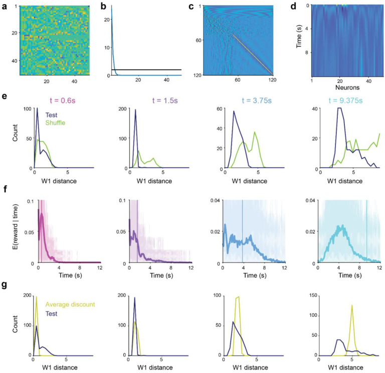
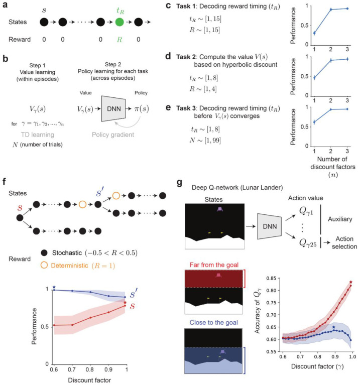
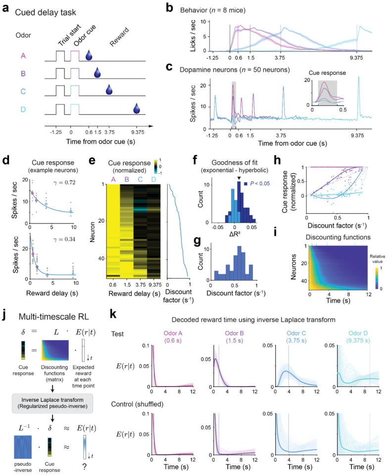
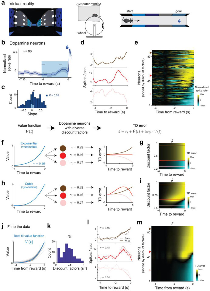
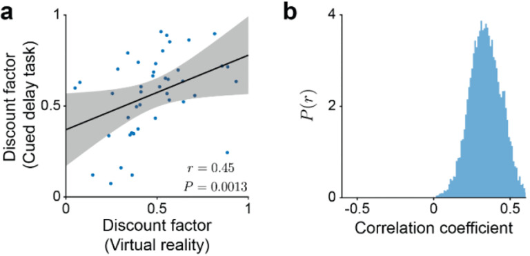
To thrive in complex environments, animals and artificial agents must learn to act adaptively to maximize fitness and rewards. Such adaptive behavior can be learned through reinforcement learning¹, a class of algorithms that has been successful at training artificial agents^2-6 and at characterizing the firing of dopamine neurons in the midbrain^7-9. In classical reinforcement learning, agents discount future rewards exponentially according to a single time scale, controlled by the discount factor. Here, we explore the presence of multiple timescales in biological reinforcement learning. We first show that reinforcement agents learning at a multitude of timescales possess distinct computational benefits. Next, we report that dopamine neurons in mice performing two behavioral tasks encode reward prediction error with a diversity of discount time constants. Our model explains the heterogeneity of temporal discounting in both cue-evoked transient responses and slower timescale fluctuations known as dopamine ramps. Crucially, the measured discount factor of individual neurons is correlated across the two tasks suggesting that it is a cell-specific property. Together, our results provide a new paradigm to understand functional heterogeneity in dopamine neurons, a mechanistic basis for the empirical observation that humans and animals use non-exponential discounts in many situations^10-14, and open new avenues for the design of more efficient reinforcement learning algorithms.

Extended Data Fig. 1 |. Decoding simulations for multi-timescale vs. single-timescale agents. (a-c).

Experiment corresponding to Fig. 2c. (decoding reward timing). a, MDP with reward $R$ at time $t_R$. b, Diagram of the decoding experiment. In each episode, the reward magnitude and time are randomly sampled from discrete uniform distributions, which defines the MDP in a. Values are learned until near convergence using TD-learning. Values with different discount factors are learned independently. The learned values for the cue ($s$) are fed into a non-linear decoder which learns, across MDPs, to report the reward time. c, Decoding performance as the decoder is trained. Different colors indicate the discount factors used in TD-learning. (d-f). Experiment corresponding to Fig. 2d. (Decoding value with hyperbolic discount). d, MDP with reward $R$ at time $t_R$. e, Diagram of the decoding experiment. In each episode, the reward magnitude and time are randomly sampled from discrete uniform distributions, which defines the MDP in d. Values are learned until near convergence using TD-learning. Values with different discount factors are learned independently. The learned values for the cue ($s$) are fed into a non-linear decoder which learns, across MDPs, to report the hyperbolic value of the cue. f, Decoding performance as the decoder is trained. Different colors indicate the discount factors used in TD-learning. (g-i). Experiment corresponding to Fig. 2e. (decoding reward timing before convergence). g, MDP with reward equal to 1 at time $t_R$. h, Diagram of the decoding experiment. In each episode, the reward time and the number of TD iterations $\left(N\right)$ are sampled from discrete uniform distributions. Values are learned by performing N TD-learning backups on the MDP. Values with different discount factors are learned independently. The learned values for the cue ($s$) are fed into a non-linear decoder which learns, across MDPs, to report the reward time. i, Decoding performance as the decoder is trained. Different colors indicate the discount factors used in TD-learning. (j-l). Decoding reward timing in a more complex task. j, MDP with two rewards of magnitude $R1$ and $R2$ at times $t_{R1}$ and $t_{R2}$. k, Diagram of the decoding experiment. In each episode, both reward magnitudes and times are sampled from discrete uniform distributions. The learned values for the cue ($s$) are fed into a non-linear decoder which learns, across MDPs, to report both reward times. l, Decoding performance as the decoder is trained. Different colors indicate the discount factors used in TD-learning. (m-o). Decoding length of branches in an MDP during training. m, MDP with two possible trajectories. In this example, the upwards trajectory is longer than the downwards trajectory. n, Diagram of the decoding experiment. In each episode, the length of the two branches D and the number of times that TD-backups are performed for each branch are randomly sampled from uniform discrete distributions. Then, TD-backups are performed for the two branches the corresponding number of times. After this, they are fed into a decoder which is trained, across episodes, to report the shorter branch. o, Decoding performance as the decoder is trained. Different colors indicate the discount factors used in TD-learning. In panels c, f, i, k and o, the shaded area corresponds to the standard deviation of the estimate over 2 repeats and smoothed of 100 episodes.

Extended Data Fig. 2 |. Temporal estimates are available before convergence for multi-timescale agents.

a, Two experiments, one with a short wait between the cue and reward (pink), and one with a longer wait (cyan). b, The identity of the cue with the higher value for a single-timescale agent (here $\gamma =0.9$) depends on the number of times that the experiments have been experienced. When the longer trajectory has been experienced significantly more often than the short one, the single-timescale agent can incorrectly believe that it has a larger value. c, For a multi-timescale agent, the pattern of values learned across discount factors is only affected by a multiplicative factor that depends on the learning rate, the prior values and the asymmetric learning experience. The pattern therefore contains unique information about outcome time. d,e, When plotted as a function of the number of times that trajectories are experienced, the pattern of values across discount factors is only affected by a multiplicative factor. In other words, for the pink cue, the larger discount factors are closer together than they are to the smaller discount factor, and the opposite for the cyan cue. This pattern is maintained at every point along the x-axis, and therefore is independent of the asymmetric experience, and it enables a downstream system to decode reward timing.

Extended Data Fig. 3 |. Myopic learning bias.

a, Maze to highlight the myopic learning bias. Rewards are indicated with water and fire. An example trajectory is shown with transparent arrows. The red and blue bars to the right denote the states in the Lower and Upper half. b, True (grey) and estimated (green and brown) values for the example trajectory on top and shown in panel a. In the x-axis we highlight the starting timestep with $s$, the timestep when the fire is reached and the timestep when the water is reached. c, Accuracy (y-axis) is measured as the Kendall tau coefficient between the estimate with a specific gamma (x-axis) and the true value function $V_{\gamma }=0.99$. Error bars are deviations across 300 sets of sampled trajectories. The red (blue) curve shows average accuracy for the states on the upper (lower) half of the maze, indicated with color lines on panel a. d, As the sampled number of trajectories increases, the myopic learning bias disappears.

Extended Data Fig. 4 |. Single neuron responses and robustness of fit in the cued delay task.

a, PSTHs of single selected neurons $(n=50)$ responses to the cues predicting a reward delay of 0.6s, 1.5s, 3.75s, and 9.375s (from top to bottom). Neurons are sorted by the inferred value of the discount factor γ. Neural responses are normalized by z-scoring each neuron across its activity to all 4 conditions. b, PSTHs of single non-selected neurons $(n=23$) responses to the cues predicting a reward delay of (from top to bottom). Neurons are sorted by the inferred value of the discount factor γ. Neural responses are normalized by z-scoring each neuron across its activity to all 4 conditions. c, Variance explained for training vs testing data for the exponential model. For each bootstrap, the variance explained was computed on both the half of the trials used for fitting (train) and the other half of the trials (test). Neurons ($n=13$) with a negative variance explained on the test data are excluded from the decoding analysis (grey dots). d, Same as panel c but for the fits for the hyperbolic model. e, Goodness of fit on held-out data for each selected neuron for the exponential and hyperbolic models. The data lies above the diagonal line suggesting a better fit from the exponential model as shown in Fig. 3f. Error bars indicate 95% confidence interval using bootstrap. f, The values of the inferred parameters in the exponential model are robust across bootstraps. top row, Inferred value of the parameters across two halves of the trials (single bootstrap) for the gain $\alpha$, baseline b and discount factor γ respectively. Bottom row, Distribution across $n=100$ bootstraps of the Pearson correlations between the inferred parameter values in the two halves of the trials for the gain α (mean = 0.84, $P<1\times {10}^{-20}$), baseline b (v, mean = 0.9, $P<1.0\times {10}^{-32}$) and discount factor γ (vi, mean =0.93, $P<1.0\times {10}^{-46}$). g, Same as panel e but for the hyperbolic model with distribution of correlations for the gain α (mean=0.86,$\mathrm{ }\mathrm{p}<1{\mathrm{e}}^{-26}$), baseline b (v, mean = 0.88, P <1.0 × 10⁻²⁸) and shape parameter k (vi, mean = 0.76, $P<1.0\times {10}^{-11}$). h, Same as panel e and g but for the exponential model simulated responses with distribution of correlations for the gain α (mean = 0.86, $P<1.0\times {10}^{-10}$), baseline b (v, mean = 0.88, $P<1.0\times {10}^{-24}$) and discount factor γ (vi, mean = 0.76, $P<1.0\times {10}^{-26}$). Note that the distributions of inferred parameters are in a similar range than the fits to the data suggesting that trial numbers constrain the accuracy of parameter estimation. Significance is the highest $p$-value for all the bootstraps for a given parameters assessed via $t$-test.

Extended Data Fig. 5 |. Decoding reward timing using the regularized pseudo-inverse of the discount matrix.

(a-c), Singular value decomposition (SVD) of the discount matrix. a, left singular vectors (in the neuron space). b, Singular values. The black line at 2 indicates the values of the regularization term α. c, right singular vectors (in the time space). d, Decoding matrix based on the regularized pseudo-inverse. e, Distribution of 1-Wassertein distances between the reward timing and the predicted reward timing from the decoding on the test data exponential fits (shown in Fig. 3k, top row) and on the shuffled data (shown if Fig. 3k, bottom row). The prediction from the test data are better predictions (smaller 1-Wasserstein distance) than shuffled data ($P=1.2\times {10}^{-4}$ for 0.6 s reward delay, $P<1.0\times {10}^{-20}$ for the other delays, one-tailed Wilcoxon signed rank test, see Methods). f, Decoded subjective expected timing of future reward $E(r\mid t)$ using a model with a single discount factor (the mean discount factor across the population, see Methods). g, Distribution of 1-wassertein distances between the reward timing and the predicted reward timing from the decoding on the test data from exponential fits (shown in Fig. 3k, top row) and on the average exponential model (shown in f). Decoding is better for the exponential model from Fig. 3 than the average exponential model except for the shortest delay $\left(P\left(t=0.6\mathrm{s}\right)=1,P\left(t=1.5\mathrm{s}\right)<1.0\times {10}^{-31},P\left(t=3.75\right)=0.0135,P\left(t=9.375\mathrm{s}\right)<1.0\mathrm{ }\times \right.{\mathrm{ }10}^{-14}$), one-tailed Wilcoxon signed rank test, see Methods).

Extended Data Fig. 6 |. Decoding reward timing from the first to the hyperbolic model and exponential model simulations.

a, Distribution of the inferred discount parameter k across the neurons. b, Correlation between the discount factor inferred in the exponential model of the discount parameter k from the hyperbolic model $\left(r=-0.9,P<1.0\times {10}^{-30}\right.,\mathrm{ }t$-test). Note the in the hyperbolic model a larger value of k implies faster discounting hence the negative correlation. c, Discount matrix for the hyperbolic model. For each neuron we plot the relative value of future events given its inferred discount parameter. Neurons are sorted by decreasing estimated value of the discount parameter. d, Decoded subjective expected timing of future reward $E(r\mid t)$ using the discount matrix from the hyperbolic model (see Methods). e, Distribution of 1-Wassertein distances between the reward timing and the predicted reward timing from the decoding on the test data with the exponential model (shown in Fig. 3k, top row) and on the test data with the hyperbolic model (shown in d). Decoding is better for the exponential model from Fig. 3 than the hyperbolic model except for the shortest delay $\left(P\right(t=0.6\mathrm{s})=1,P(t=1.5\mathrm{s})<\left.1.0\times {10}^{-31},P(t=3.75)<1.0\times {10}^{-33},P(t=9.375\mathrm{s})<1.0\times {10}^{-3}\right)$, one-tailed Wilcoxon signed rank test, see Methods). f, Decoded subjective expected timing of future reward $E(r\mid t)$ using simulated data based on the parameters of the exponential model (see Methods). g, Distribution of 1-Wassertein distances between the reward timing and the predicted reward timing from the decoding on the test data from exponential fits (shown in Fig. 3k, top row) and on the simulated data from the parameters of the exponential fits (shown in f). Decoding is marginally better for the data predictions $\left(P\right(t=0.6\mathrm{s})=0.002,\left.P(t=1.5\mathrm{s})=0.999,P(t=3.75)<1\times {10}^{-12},P(t=9.375\mathrm{s})=0.027\right)$, one-tailed Wilcoxon signed rank test, see Methods), suggesting that decoding accuracy is limited by the number of trials.

Extended Data Fig. 7 |. Ramping, discounting and anatomy.

a, Ramping in the prediction error signal is controlled by the relative contribution of value increases and discounting. If the value increase (middle) exactly matches the discounting, there is no prediction error (middle equation, right). If the discounting is smaller than the value increase (large discount factor) then there is a positive TD error (top equation, right). If the discounting is larger (small discount factor) than the value increase then there a negative TD error (bottom equation, right). A single timescale agent with no state uncertainty will learn an exponential value function but if there is state uncertainty (see ref[]) or the global value function arises from combining the contribution of single-timescale agents then the value function is likely t be non-exponential. b, The discount factor inferred in the VR task is not correlated with the medio-lateral (ML) position of the implant (Pearson’s $r=0.015,P=0.89$). c, The baseline parameter inferred in the VR task is not correlated with the medio-lateral (ML) position of the implant (Pearson’s $r$ $=-0.011,P=0.92)$. d, The inferred gain in the VR task reduces with increasing medio-lateral (ML) position but the effect does not reach significance (Pearson’s $r=-0.19,P=0.069$).

Extended Data Fig. 8 |. Discounting heterogeneity explains ramping diversity in a common reward expectation model.

a, Uncertainty in reward timing reduces as mice approach the reward zone. Not only does the mean expected reward time reduces but the standard deviation of the estimate also reduces. Distribution in the bottom row from fitted data (see panels c-i). b, Simulations showing how reduction in uncertainty in reward timing (shared across neurons) and diverse discount factors lead to heterogeneous ramping activity in dopamine neurons. First panel. In this model, the uncertainty in the subjective estimate of reward timing (measured by the standard deviation) reduces as the mice approach the reward. Second panel. Distribution of subjective expected time to reward as a function of the true time to reward. The distribution is sampled from a folded normal distribution. The standard deviation reduces as reward approaches as shown in the first panel. Third panel. Given the subjective expected time to reward, common to all neurons due to a single world mode, we can compute a value function for each neuron given its discount factor. Fourth panel. This leads to a heterogeneity of TD errors across neurons, including monotonic upward and downwards ramps as well as non-monotonic ramps. c, The inferred standard deviation of the reward expectation model reduces as a function of time to reward. Line indicates the mean inferred standard deviation and the shading indicates the standard error of the mean over 100 bootstraps. d, Subjective expected timing of the reward as a function of true time to reward. As the mice approach the reward not only does the mean expected time to reward reduces but the uncertainty of the reward timing captured by the standard deviation shown in c also reduces. This effect leads to increasingly convex value functions that lead to the observed ramps in dopamine neuron activity. e, Value function for each individual neuron. f, Distribution of inferred discount factors under the common reward expectation model. g, Although the range of discount factor between the fits from the common value (x-axis) and common reward expectation (y-axis) models differs, the inferred discount factors are strongly correlated for single neurons (Spearman’s $\rho =0.93,P<1.0\times {10}^{-20}$). h, Predicted ramping activity from the model fits under the common reward expectation model. i, Diversity of ramping activity across single neurons as mice approach reward (aligned by inferred discount factor in the common reward expectation model).

Extended Data Fig. 9 |. Decoding reward timing in the cud delayed reward task using parameters inferred in the VR task.

a, Discount matrix computed using the parameters inferred in the VR tasks for neurons recorded across both tasks and used in the cross-task decoding. b, Dopamine neurons cue responses in the cued delay task. Neurons are aligned as in a according to increasing discount factor inferred in the VR task. c, Top row: Decoded reward timing using discount factors inferred in the VR task. Bottom row: The ability to decode reward timing is lost when shuffling the identities of the cue responses. d, Except for the shortest delay, decoded reward timing is more accurate than shuffle as measured by the 1-Wassertsein distance $\left(P_{t=0.6\mathrm{s}}=1,P_{t=1.5\mathrm{s}}<1.1\times {10}^{-20},P_{t=3.75\mathrm{s}}<3.8\times {10}^{-20},P_{t=9.375\mathrm{s}}\right.\left.\mathrm{ }<2.9\times {10}^{-5}\right)$.

Figure 1 |. Single timescale and multi-timescale reinforcement learning.

a, In single-timescale value learning, the value of a cue (at $t=0$) predicting future rewards (first panel) is evaluated by discounting these rewards with a single exponential discounting function (second panel). The expected reward size and timing are encoded, but confounded, in the value of the cue (third panel). b, In multi-timescale value learning, the same reward delays are evaluated with multiple discounting functions (second panel). The relative value of a cue as a function of the discount depends on the reward delay (third panel). A simple linear decoder based on the Laplace transform can thus reconstruct both the expected timing and magnitude of rewards (fourth panel).

Fig. 2 |. Computational advantages of multi-timescale reinforcement learning.

a, Experiment to compare single- vs. multi-timescale learning. b, Architecture to evaluate multi-timescale advantages. In each episode (defined by a specific $R,t_R$ and $N$) the value function is learned via tabular updates. The policy gradient network is trained across episodes to maximize the accuracy of the report. c, The timing $t_R$ and reward size $R$ is varied across episodes, the task of the policy gradient (PG) network is to report $t_R$. d, The timing $t_R$ and reward size $R$ is varied across episodes, the task is to report the inferred value of s using a hyperbolic discount. e, The timing $t_R$ and number of sampled trajectories $N$ is varied across episodes, the task of the policy gradient (PG) network is to report $t_R$. In c-e, Performance is reported after 1,000 training episodes. Error bars are the standard deviations (s.d.) across 100 test episodes and 3 trained policy gradient (PG) networks. f, Myopic learning bias. Top: Task structure to evaluate the learning bias induced by the discount factor, the three dots collapse 5 transitions between black states. Bottom: Performance at selecting the branch with the large deterministic reward under incomplete learning conditions. At state s (orange), agents with larger discount factors (far-sighted) are more accurate. At state s’ (blue), agents with a small discount factor (myopic) are more accurate. Error bars are half s.d. across 10,000 episodes, maximums are highlighted with stars. g, Top: Architecture that learns about multiple timescales as auxiliary tasks. Bottom: Accuracy of the Q-values in the Lunar Lander environment as a function of their discount factor, estimated as the fraction of concordant state pairs between the empirical value function and the discount specific Q-value estimated by the network, when the agent is close to the goal (blue) or far from the goal (orange), see Methods for details. Error bars are s.e.m across 10 trained networks, maximums are highlighted with stars.

Figure 3 |. Dopamine neurons exhibit a diversity of discount factors that enables decoding of reward delays.

a, Outline of the task structure. b, The mice exhibit anticipatory licking prior to reward delivery for all 4 reward delays indicating that they have learned task contingencies (mean across behavior for all recorded neurons, shaded error bar indicates 95% confidence interval using bootstrap). c, Average PSTH across the task for the 4 trial types. Inset shows the firing rate in the 0.5s following the cue predicting reward delay. The firing rate in the shaded grey box $(0.1s<t<0.4s)$ was used as the cue response in subsequent analysis. d, Example of fits of the responses to the cue predicting reward delay of two single neurons with high (top panel) and low (bottom panel) discount factors. e, Normalized response to the cues predicting reward delays across the population. For each neuron, the response was normalized to the highest response across the 4 possible delays. Inset on right, corresponding inferred discount factor for each neuron. f. The exponential model is a better fit to the data than the hyperbolic one as quantified by distance of mean $R^2$ to the unit line. Mean = 0.0147, $P=2.2\times {10}^{-5}$, two-tailed $t$-test. Shading indicated significance for single neurons across bootstraps (dark blue: $P<0.05$). g, Distribution of inferred discount factors across neurons. For each neuron, the discount factor was taken as the mean discount factor across bootstraps. h. Shape of the relative population response as a function of reward delay. Normalized to the strongest cue response for each neuron. Thick lines, smoothed fit, dotted lines, theory, dots, responses of individual neurons. i, Discount matrix. For each neuron we plot the relative value of future events given its inferred discount factor. Neurons are sorted as in panel d by increasing inferred value of the discount factor. Vertical bars on top of panel are color coded to indicate timing of the rewards in the task. j, Outline of the decoding procedure. We compute the singular value decomposition (SVD) of the discount matrix L. Then, we use the SVD to compute a regularized pseudo-inverse ${\mathit{L}}^{-1}$. Finally, we normalize the resulting prediction into a probability distribution. k, The subjective expected timing of future reward $E(r\mid t)$ can be decoded from the population responses to the cue predicting reward delay. Decoding based on mean cue responses for test data (top row, see Methods). The ability to decode the timing of expected future reward is not due to a general property of the discounting matrix and collapses if we randomize the identity of the cue responses (bottom row, see Extended Data Fig. 5e and Methods).

Figure 4 |. The diversity of discount factors across dopamine neurons explains qualitatively different ramping activity.

a, Experimental setup. Left panel, View of the virtual reality corridor at movement initiation. Middle and right, Schematics of the experimental setup. b, Average activity of single dopaminergic neurons $(n=90$) exhibit an upward ramp in the last few seconds of the track prior to reward delivery. c, The slope of the activity ramp (computed between the two black horizontal ticks in panel b) is positive on average but varies across neurons (population: mean slope = 0.097, $P=0.0175$. Single neurons: positive and $P<0.05: n=53$; negative and $P<0.05:n=32;P>0.05:n=5$, two-tailed $t$-test). d, Example single neurons showing diverse ramping activity in the final approach to reward including, monotonic upwards (dark red), non-monotonic (red) and monotonic downwards (light red) ramps. e, Individual neurons across the population exhibit a spectrum of diversity in their ramping activity. Neurons are sorted according to inferred discount factor from the common value function model (panel k). f, Diversity of ramping with an exponential value function. There is no TD error for an agent with the same discount factor as the parameter of the value function (red line). The TD error ramps upwards (downwards) if the discount factor is larger (smaller), dark red and light red lines respectively. g, Diversity of ramping as a function of discount factor for an exponential value function. h, Diversity of ramping with cubic value function. Agents with large (small) discount factor experience a monotonic positive (negative) ramp in their TD error (dark red and light red lines respectively). Agents with intermediate discount factors experience non-monotonic ramps (red line). i, Diversity of ramping as a function of discount factor for an exponential value function. Unlike in the exponential value function case, no agent matches its discount to the value function at all the time steps. j, The inferred value function is convex. Thin grey lines represent the inferred value function for each bootstrap. Thick blue line represents mean over bootstraps. k, Histogram of inferred discount factors. 0.42 ± 0.23 (mean ± s.d.). l, Example model fits for the single neurons shown in panel d. m, The model captures the diversity of ramping activity across the population. Neurons are ordered by inferred discount factor as in panel e.

Figure 5 |. Discount factors of single dopaminergic neurons are correlated across behavioral contexts.

a, Correlation between the discount factors inferred in the VR task and the discount factors inferred in the cued delay task ($r=0.45,P=0.0013)$. b, Distribution of correlations between the discount factors across the two tasks for randomly sampled pairs of bootstrap estimates (0.34 ± 0.104, mean ± s.d., $P<1.0\times {10}^{-30}$, two-tailed t-test)

References

1. Sutton R. S. & Barto A. G. Reinforcement Learning: An Introduction (Adaptive Computation and Machine Learning series). 552 (A Bradford Book, 2018).
1. Tesauro G. Temporal difference learning and TD-Gammon. Commun. ACM 38, 58–68 (1995).
1. Mnih V. et al. Human-level control through deep reinforcement learning. Nature 518, 529–533 (2015). - PubMed
1. Silver D. et al. Mastering the game of Go with deep neural networks and tree search. Nature 529, 484–489 (2016). - PubMed
1. Ecoffet A., Huizinga J., Lehman J., Stanley K. O. & Clune J. First return, then explore. Nature 590, 580–586 (2021). - PubMed
Publication types