Multimodal subspace identification for modeling discrete-continuous spiking and field potential population activity

Abstract

Objective.Learning dynamical latent state models for multimodal spiking and field potential activity can reveal their collective low-dimensional dynamics and enable better decoding of behavior through multimodal fusion. Toward this goal, developing unsupervised learning methods that are computationally efficient is important, especially for real-time learning applications such as brain-machine interfaces (BMIs). However, efficient learning remains elusive for multimodal spike-field data due to their heterogeneous discrete-continuous distributions and different timescales.Approach.Here, we develop a multiscale subspace identification (multiscale SID) algorithm that enables computationally efficient learning for modeling and dimensionality reduction for multimodal discrete-continuous spike-field data. We describe the spike-field activity as combined Poisson and Gaussian observations, for which we derive a new analytical SID method. Importantly, we also introduce a novel constrained optimization approach to learn valid noise statistics, which is critical for multimodal statistical inference of the latent state, neural activity, and behavior. We validate the method using numerical simulations and with spiking and local field potential population activity recorded during a naturalistic reach and grasp behavior.Main results.We find that multiscale SID accurately learned dynamical models of spike-field signals and extracted low-dimensional dynamics from these multimodal signals. Further, it fused multimodal information, thus better identifying the dynamical modes and predicting behavior compared to using a single modality. Finally, compared to existing multiscale expectation-maximization learning for Poisson-Gaussian observations, multiscale SID had a much lower training time while being better in identifying the dynamical modes and having a better or similar accuracy in predicting neural activity and behavior.Significance.Overall, multiscale SID is an accurate learning method that is particularly beneficial when efficient learning is of interest, such as for online adaptive BMIs to track non-stationary dynamics or for reducing offline training time in neuroscience investigations.

Keywords: Poisson and Gaussian data; dynamical systems; local field potentials; multimodal data; spiking activity; unsupervised learning.

Figure 1.

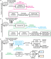
Multiscale SID algorithm for modeling and prediction of neural activity and behavior. (a) The traditional covariance-based SID algorithm learns the single-scale model parameters from a continuous modality (e.g. field potentials) in the training set (magenta box). These parameters are extracted from the future–past cross-covariance of the continuous modality H _y , which can be computed directly from its observations. (b) The new multiscale SID algorithm (see algorithms 1 and 2) learns the multiscale model parameters from the discrete-continuous modalities (e.g. spike-field activity) in the training set (green box). Given that firing rates are latent, future–past cross-covariance of log firing rates and continuous modality H _w is not directly computable from the multimodal observations. Instead, we compute this cross-covariance H _w by transforming the moments of the discrete-continuous observations using the multiscale model equations. Then, we estimate the multiscale model parameters from H _w via SID methods. However, covariance-based SID methods even for a single modality do not guarantee valid noise statistics. We address this challenge by imposing added constraints in our SID method to enforce valid noise statistics within a novel optimization formulation. These constraints are critical for enabling multiscale statistical inference of latent states. (c) The learned valid parameter set is used to infer the latent states using a multiscale filter in the test set. These states are then used to predict behavior and the discrete-continuous neural activity using the learned model. (d) After learning the model parameters, the dynamical modes corresponding to a pair of complex conjugate eigenvalues or a real eigenvalue of A are computed.

Figure 2.

Multiscale SID accurately identifies the model parameters in simulations. Normalized identification error of all parameters in multiscale SID as a function of number of training samples across 50 randomly generated multiscale models. All parameter identification errors decrease as more training samples are used. Using 10⁶ samples, all normalized errors are less than $6\mathrm{\%}$. The dashed horizontal line indicates $6\mathrm{\%}$ normalized error. The normalized error is the Frobenius norm of the difference between the true and identified parameters, which is then normalized by the true parameter norm (equation (42)). Solid lines show the mean and shaded area represents s.e.m. The set $\{\mathbf{A},{\mathbf{C}}_z,{\mathbf{C}}_y,{\mathbf{G}}_z,{\mathbf{G}}_y,{\mathrm{\Lambda }}_0,{\mathbf{d}}_z\}$ fully characterize the multiscale model in equation (1), where ${\mathrm{\Lambda }}_0=\mathrm{C}\mathrm{o}\mathrm{v}[(\begin{array}{cc}{\mathbf{z}}_t^{\mathrm{\prime }}& {\mathbf{y}}_t^{\mathrm{\prime }}\end{array}{)}^{\mathrm{\prime }}]$ is the covariance of concatenated log firing rates and field potential signals, and ${\mathbf{G}}_y=\mathrm{C}\mathrm{o}\mathrm{v}[{\mathbf{x}}_{t+1},{\mathbf{y}}_t]$ and ${\mathbf{G}}_z=\mathrm{C}\mathrm{o}\mathrm{v}[{\mathbf{x}}_{t+1},{\mathbf{z}}_t]$ are the cross-covariances of latent states with log firing rates and field potential signals, respectively (see sections 2.2.5 and 2.3.2).

Figure 3.

Multiscale SID outperforms multiscale EM in training time and identification of dynamical modes in simulations. (a) Training time (in seconds) of multiscale SID and multiscale EM with different number of iterations as a function of number of training samples. Multiscale SID has a much lower training time compared with multiscale EM. Also, the training time of multiscale EM monotonically increases with more iterations or training samples. Solid line represents the mean across 50 simulated models and shaded area represents s.e.m. (b) Training time of multiscale SID vs multiscale EM using $5\times {10}^4$ training samples (indicated by vertical dashed line on panel (a)). This training sample size has the same order of magnitude as the NHP dataset. Bars represent the median, box edges represent 25th and 75th percentiles, and whiskers show the minimum and maximum values (other than outliers). Outliers are the points that are more than 1.5 times the interquartile distance (the box length) away from the top and bottom of the box. The dots represent individual data points. Asterisks indicate significance of performance comparison between multiscale SID and multiscale EM. (Wilcoxon signed rank test, $N_{\mathrm{s}}$ = 50, *: P < 0.05, **: P < 0.005, ***: P < 0.0005). (c) For one simulated multiscale model, the true and SID identified eigenvalues of the state transition matrix A are shown in black and green circles for $2\times {10}^3$ (left) and $5\times {10}^4$ training samples (right). Red lines indicate the identified eigenvalue errors, that is mode errors. Each dynamical mode corresponds to a pair of complex conjugate or a real eigenvalue of the true state transition matrix A (figure 1(d)). Normalized mode error is computed by first dividing the sum of the squared length of the red error lines by the sum of the true eigenvalue squared magnitude, and then taking its square root (section 2.3.2). Normalized mode error decreases with increasing the training sample size. (d) and (e) Same as (b) and (c) but for normalized mode error. Multiscale SID has a significantly lower mode error compared with multiscale EM. The normalized mode error monotonically decreases with more iterations for multiscale EM and with more training samples for both multiscale EM and SID.

Figure 4.

While allowing for significantly faster training time (figure 3), multiscale SID still has comparable performance to multiscale EM in predicting spiking and field potential data in simulations. (a) One-step-ahead prediction accuracy of field potential activity quantified by correlation coefficient (CC) between the one-step-ahead predicted and the true field potential activity for multiscale SID and multiscale EM (with different number of iterations) as a function of training samples. (b) One-step-ahead prediction performance of field potential activity for multiscale SID vs multiscale EM using $5\times {10}^4$ training samples, which is similar to the number of samples in the NHP datasets and indicated by the vertical dashed line on panel (a). (c) and (d) Same as (a) and (b) but for one-step-ahead prediction accuracy of spiking activity quantified by prediction power (PP, section 2.3.4). Figure convention is as in figure 3, and the performance is also reported for the same 50 simulated systems in that figure ($N_{\mathrm{s}}=50$). Overall, multiscale SID performs similarly in neural prediction to multiscale EM in simulations when enough training samples—but still comparable to that of the real data—are available.

Figure 5.

Multiscale SID outperforms single-scale SID in identification of dynamical modes in simulations due to fusion of information across modalities, with the largest performance gain being obtained in the low information regime. (a) Normalized mode error (section 2.3.2) as increasingly more continuous field potential signals are gradually combined with 4, 6, or 14 baseline discrete spiking signals. The start of the curves (i.e. 0 on x-axis) indicates normalized mode error for single-modal signals (i.e. spiking signals only). Solid line indicates mean across 50 simulated neural network systems and shaded area represents s.e.m ($N_{\mathrm{s}}=50$ data points). (b) Comparison of the maximum improvement of normalized mode error after combining continuous field potential signals with 4, 6, or 14 baseline discrete spiking signals. Bars represent the median and box conventions are the same as in figure 3. Dots represent individual data points. Asterisks indicate significance of a pairwise comparison of improvement value across baseline regimes as well as comparison of improvement value with 0 (Wilcoxon signed rank test, $N_{\mathrm{s}}=50$, ***: P < 0.0005). (c) and (d) Same as (a) and (b) but for gradually combining increasingly more spiking signals with a fixed number of baseline field potential signals.

Figure 6.

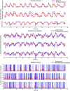
Prediction of example behavior trajectories, field potential and spiking activity in one test fold of NHP datasets. We learn the multiscale model using multiscale SID with $n_x=24$ in the training data and use it in the test data to extract the latent states and predict behavior and spike-LFP activity from these states (see sections 2.3.4, 2.4.3 and 2.4.4). (a) Example joint angle time-series and their predictions. (b) Example field potential power feature time-series and their one-step-ahead predictions. (c) Example spike events and their one-step-ahead predicted probability (probability of having at least one spiking event in the 10 ms time bin). This predicted probability is expected to be higher when more spiking events are occurring. Each vertical blue line indicates the time of one spike event.

Figure 7.

In NHP datasets, multiscale SID outperforms multiscale EM in both training time and neural prediction accuracy and matches the accuracy of multiscale EM in prediction of behavior. (a) Spike-LFP activity was recorded as a non-human primate performed naturalistic reach and grasp movements to randomly positioned objects in 3D space. (b) Left: training time (in seconds) of multiscale SID and multiscale EM with different number of iterations as a function of latent state dimension. Training time monotonically increases with more multiscale EM iterations or latent state dimensions. Solid line represents the mean and shaded area represents s.e.m. over folds and data sessions ($N_{\mathrm{s}}=35$ data points). Right: comparison of training time of multiscale SID and that of multiscale EM at $n_x=24$. Multiscale SID is significantly faster, approximately 30 times faster than multiscale EM. Bar, box and asterisks conventions are as in figure 3. (c) and (d) Same as left panel of (b) but for one-step-ahead prediction accuracy of field potentials (quantified by correlation coefficient (CC), section 2.3.4), one-step ahead prediction accuracy of spiking activity (quantified by prediction power (PP), section 2.3.4), and behavior prediction accuracy (quantified by CC, section 2.4.3).

Figure 8.

In NHP datasets, multiscale SID improves the behavior prediction accuracy compared to single-scale SID due to fusion of information across modalities and this improvement is largest in the low information regime. (a) Behavior prediction accuracy quantified by correlation coefficient (CC) between the predicted and true behavior as increasingly more field potential signals are combined with to 2 (blue), 6 (red) and 14 (yellow) baseline spiking signals. The start of the curves (i.e. 0 on x-axis) indicates behavior prediction for single-modal neural activity (i.e. spiking signals only). Solid line indicates mean across folds, random sets of selected neural signals and data sessions and shaded area represents s.e.m ($N_{\mathrm{s}}=350$ data points). (b) Comparison of the maximum improvement of behavior prediction (quantified by difference of CCs) after combining field potential signals with 2 (blue), 6 (red) and 14 (yellow) spiking signals (section 2.4.6). Bars indicate median and box conventions are as in figure 3. Dots represent individual data points. Asterisks indicate significance of a pairwise comparison of improvement value across baseline regimes as well as comparison of improvement value with 0 (Wilcoxon signed rank test, $N_{\mathrm{s}}=350$, ***: P < 0.0005). (c) and (d) Same as (a) and (b) but for combining increasingly more spiking signals with a fixed number field potential signals (baseline field potential signals).

Figure A1.

The optimization problem satisfies the desired conditions. Normalized norm of parameters R _z , ${\mathbf{R}}_{zy}$ and S (defined in section 2.3.3) identified by multiscale SID as a function of number of training samples across 50 randomly generated multiscale models. All normalized norms decrease as more training samples are used. Using 10⁶ samples, all normalized norms are less than $6\mathrm{\%}$. The dashed horizontal line indicates $6\mathrm{\%}$ normalized norm. Since R _y is not in the cost function, its normalized norm is shown as a control to show that it is not driven to zero. Solid lines show the mean and shaded area represents s.e.m.

Figure A2.

Multiscale SID (compared to single-scale SID) improves the identification of collective dynamics in both modalities. (a) Normalized errors of shared modes (blue) and distinct field modes (orange) that are only present in the field potential activity, as increasingly more field potential signals combined with six spiking signals. The start of the curves (i.e. 0 on x-axis) indicate normalized mode error for single-modal signals (i.e. spiking signals only). Solid line indicates mean across 50 simulated neural network activities and shaded area represents s.e.m. (b) same as (a) but for combining increasingly more spiking signals with six field potential signals. These simulation results suggest that multiscale SID correctly combines information across modalities of neural activity.

Figure A3.

The contribution of dynamical modes to LFP activity, spiking activity, and behavior and their correlation quantified by Pearson correlation coefficient (CC). The behavior predictive modes are shown by red dots. Dots correspond to modes identified by multiscale SID using latent state dimension $n_x=14$ in 5 folds and 7 data sessions, and the dot sizes are proportional to the mode contributions to behavior prediction. The grey line is the least squares fitted line to the dots in each panel. Asterisks indicate significance of Pearson’s CC between contributions of modes in different modalities ($N_{\mathrm{s}}$ = 312, ***: P < 0.0005).

References

1. Mazor O, Laurent G. Transient dynamics versus fixed points in odor representations by locust antennal lobe projection neurons. Neuron. 2005;48:661–73. doi: 10.1016/j.neuron.2005.09.032. - DOI - PubMed
1. Wu W, Kulkarni J E, Hatsopoulos N G, Paninski L. Neural decoding of hand motion using a linear state-space model with hidden states. IEEE Trans. Neural Syst. Rehabil. Eng. 2009;17:370–8. doi: 10.1109/TNSRE.2009.2023307. - DOI - PMC - PubMed
1. Yu B, Cunningham J, Santhanam G, Ryu S, Shenoy K, Sahani M. Gaussian-process factor analysis for low-dimensional single-trial analysis of neural population activity. J. Neurophysiol. 2009;102:614–35. doi: 10.1152/jn.90941.2008. - DOI - PMC - PubMed
1. Lawhern V, Wu W, Hatsopoulos N, Paninski L. Population decoding of motor cortical activity using a generalized linear model with hidden states. J. Neurosci. Methods. 2010;189:267–80. doi: 10.1016/j.jneumeth.2010.03.024. - DOI - PMC - PubMed
1. Truccolo W, Hochberg L R, Donoghue J P. Collective dynamics in human and monkey sensorimotor cortex: predicting single neuron spikes. Nat. Neurosci. 2010;13:105–11. doi: 10.1038/nn.2455. - DOI - PMC - PubMed
Publication types
LinkOut - more resources