Exploring the dynamics of intentional sensorimotor desynchronization using phasing performance in music

Abstract

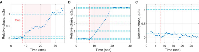
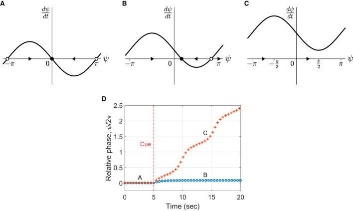
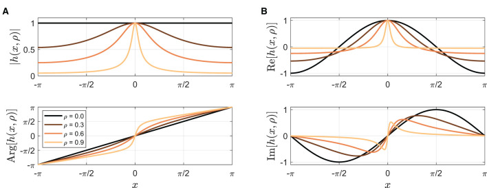
Humans tend to synchronize spontaneously to rhythmic stimuli or with other humans, but they can also desynchronize intentionally in certain situations. In this study, we investigate the dynamics of intentional sensorimotor desynchronization using phasing performance in music as an experimental paradigm. Phasing is a compositional technique in modern music that requires musicians to desynchronize from each other in a controlled manner. A previous case study found systematic nonlinear trajectories in the phasing performance between two expert musicians, which were explained by coordination dynamics arising from the interaction between the intrinsic tendency of synchronization and the intention of desynchronization. A recent exploratory study further examined the dynamics of phasing performance using a simplified task of phasing against a metronome. Here we present a further analysis and modeling of the data from the exploratory study, focusing on the various types of phasing behavior found in non-expert participants. Participants were instructed to perform one phasing lap, and individual trials were classified as successful (1 lap), unsuccessful (> 1 laps), or incomplete (0 lap) based on the number of laps made. It was found that successful phasing required a gradual increment of relative phase and that different types of failure (unsuccessful vs. incomplete) were prevalent at slow vs. fast metronome tempi. The results are explained from a dynamical systems perspective, and a dynamical model of phasing performance is proposed which captures the interaction of intrinsic dynamics and intentional control in an adaptive-frequency oscillator coupled to a periodic external stimulus. It is shown that the model can replicate the multiple types of phasing behavior as well as the effect of tempo observed in the human experiment. This study provides further evidence that phasing performance is governed by the nonlinear dynamics of rhythmic coordination. It also demonstrates that the musical technique of phasing provides a unique experimental paradigm for investigating human rhythmic behavior.

Keywords: coordination dynamics; dynamical systems; music performance; oscillator model; phasing; rhythmic coordination.

Figure 1

A phasing section from Steve Reich's Drumming (1971/2011). The basic six-beat pattern is shown in musical notation (top), and different alignments of two drummers are shown in piano-roll representations (A–C). Vertical colored lines indicate the beginning of each repetition of the pattern. (A) Two drummers' beats are aligned at the beginning of the phasing process. Drummer 2 is (B) a half beat (an eighth note) ahead of Drummer 1 in the middle and (C) one full beat (a quarter note) ahead at the end of phasing.

Figure 2

The procedure of a phasing trial.

Figure 3

Parsing of a phasing trial. The unwrapped relative phase of each tap is plotted vs. its timestamp. The vertical axis displays unwrapped relative phase divided by 2π to show the number of phasing laps clearly. In this particular trial, one phasing lap was made, with 15 taps within the phasing window. See text for details.

Figure 4

Examples of different phasing outcomes. (A) A successful trial (one phasing lap made as instructed), (B) an unsuccessful trial (more than one phasing lap; 4 laps were made in this particular trial), and (C) an incomplete trial (no complete phasing lap made).

Figure 5

(A) Box plots showing the number of taps per phasing lap for trials grouped by the total number of phasing laps (green background: successful trials, red background: unsuccessful trials). The red dots show the mean taps per lap for each group. Nine trials with more than 50 taps/lap (the max at 84 taps, all successful trials) are beyond the plotting range and not shown. (B) Success rate (the percentage of successful trials) for individual participants (N = 25) plotted against their average taps per phasing lap (for the successful and the unsuccessful trials combined). Participants with different levels of musical experience (in years of playing musical instruments) are indicated by different markers (see the legend).

Figure 6

Effect of metronome tempo. (A) The proportions of three different phasing outcomes for each metronome tempo. (B) Average taps per phasing lap in the successful and the unsuccessful trials shown for each tempo. Error bars indicate 95% confidence intervals, and dashed lines show the linear fits for the successful and the unsuccessful trials separately.

Figure 7

(A) Subtypes of incomplete trials: trapped, return, halfway, and backward. The magenta dotted lines indicate the initial in-phase range ± one width of the range, which was used to determine trapped trials. (B) The number of the subtypes of incomplete trials shown for each metronome tempo.

Figure 8

A car analogy for the dynamic landscape of phasing performance. (A) An unwrapped flat representation. The in-phase attractor is depicted as a valley. (B) The true circular landscape where phasing starts and ends at the same point. The dashed line depicts a perfect circle so that it is a valley if the ground is below the dashed line and a hill if above the dashed line.

Figure 9

Flow in the vector field defined by Equation (3) for (A) Δω = 0, (B) Δω = 0.5, and (C) Δω = 1.5 for c = 1. The arrows indicate the direction of flow. The filled and empty circles denote stable and unstable fixed points, respectively. (D) Simulations of the model with fixed detuning (Equation 2) with the parameters in (B, C). Frequency detuning is introduced at t = 5 sec. The markers indicate the (unwrapped) relative phase of individual “taps” produced by the oscillator (phase zero-crossing). Common parameter: ω₀ = 4π rad/sec (i.e., 2 Hz or 120 BPM).

Figure 10

(A) The amplitude of pulse-like function h(x, ρ) for ρ= 0, 0.3, 0.6, and 0.9 (see Appendix for the equation). (B) The coupling function f(θ, ϕ, ρ) for ρ = 0.7 (Equation 6). (C) The gating function g(θ, ϕ, ρ) when ψ > ψ_θ for ρ = 0.7 (Equation 7). The diagonal indicates where the relative phase is zero (ψ = ϕ − θ = 0).

Figure 11

Simulations of the context-dependent model (Equations 4–7): (A) successful phasing (Δ = 1 rad/sec), (B) unsuccessful phasing (Δ = 3 rad/sec), and (C) incomplete phasing (Δ = 0.5 rad/sec). The top plots show the unwrapped relative phase at the time of each “tap” (zero crossing of the wrapped oscillator phase). The bottom plots show the continuous time series of the natural frequency ω. Common parameters: c = 30, γ = 15, λ = 0 (t < 5 sec), λ = 3 (t ≥ 5 sec), ψ_θ = π/2, ω₀ = 4π rad/sec (i.e., 2 Hz or 120 BPM), and ρ = 0.7012.

Figure 12

Tempo effect in the context-dependent model. (A–C) The classification of model simulations as successful (one phasing lap), unsuccessful (more than one lap), and incomplete (0 lap). For each of seven tempi, 40,401 simulations were run for different combinations of γ and Δ (201 × 201 = 40401). Only the results for the lowest, the middle, and the highest tempi (80, 110, and 140 BPM) are shown. Dashed lines demarcate the anti-diagonal region used for Panels E and F. Parameters: c = 30, λ = 0 (before cue), λ = 3 (after cue), ψ_θ = π/2, and ρ = 0.7870 (80 BPM), 0.7643 (90 BPM), 0.7425 (100 BPM), 0.7214 (110 BPM), 0.7012 (120 BPM), 0.6817 (130 BPM), and 0.6630 (140 BPM). (D) The amplitude of the pulse-like function, |h(θ, ρ)|, plotted as function of time for different metronome tempi from 80 BPM (the lightest color) to 140 BPM (black). A different ρ was chosen for each tempo (listed above) so that the full width at half max is constant at 100 msec. (E) Simulated trial outcomes per metronome condition (only the anti-diagonal area between the dashed lines was counted). (F) Average taps per phasing lap in the “successful” and the “unsuccessful” simulations for each tempo.

Figure A1

(A) The amplitude and phase, and (B) the real and imaginary parts of the pulse function h(x, ρ) for ρ= 0, 0.3, 0.6, and 0.9.

References

1. Aschersleben G. (2002). Temporal control of movements in sensorimotor synchronization. Brain Cognit. 48, 66–79. 10.1006/brcg.2001.1304 - DOI - PubMed
1. Beek P. J., Peper C. L. E., Daffertshofer A. (2000). “Timekeepers versus nonlinear oscillators: how the approaches differ,” in Rhythm Perceptions and Productions, eds. Desain P., Windsor L.. Lisse, Netherlands: Swets & Zeitlinger, 9–33.
1. Bégel V., Demos A. P., Wang M., Palmer C. (2022). Social interaction and rate effects in models of musical synchronization. Front. Psychol. 13, 865536. 10.3389/fpsyg.2022.865536 - DOI - PMC - PubMed
1. Cohn R. (1992). Transpositional combination of beat-class sets in Steve Reich's phase-shifting music. Persp. New Music 30, 146. 10.2307/3090631 - DOI
1. deGuzman G. C., Kelso J. A. S. (1991). Multifrequency behavioral patterns and the phase attractive circle map. Biol. Cybern. 64, 485–495. 10.1007/BF00202613 - DOI - PubMed