Compact deep neural network models of visual cortex

Abstract

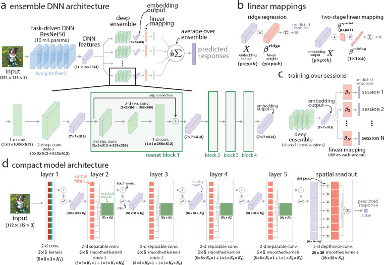
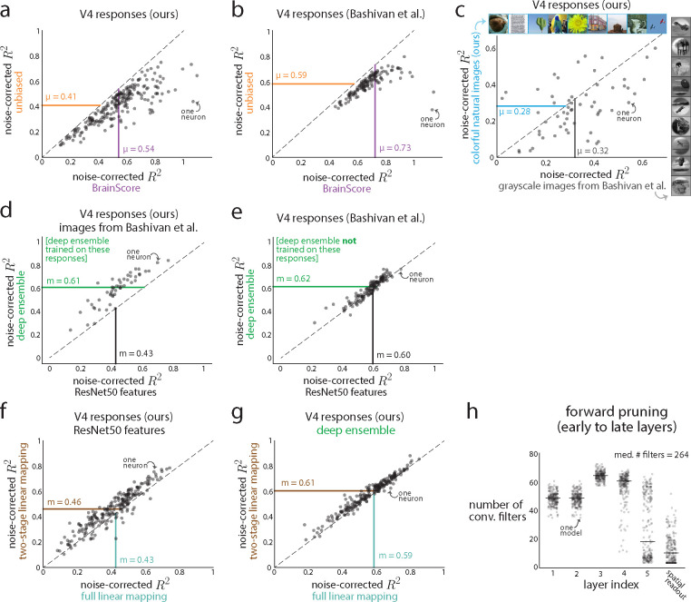
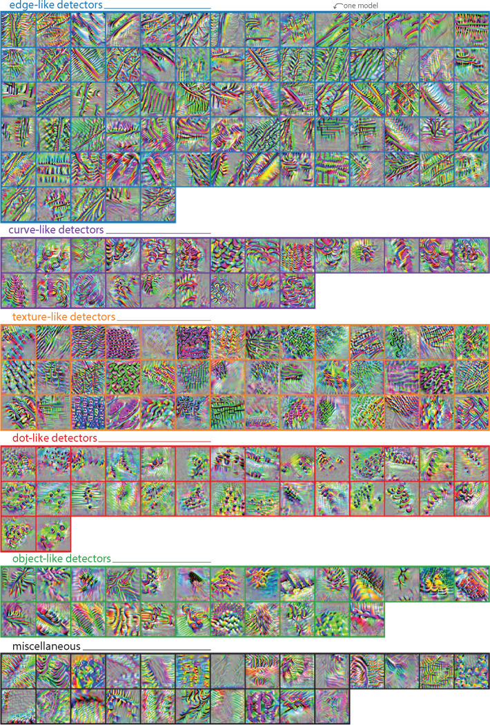
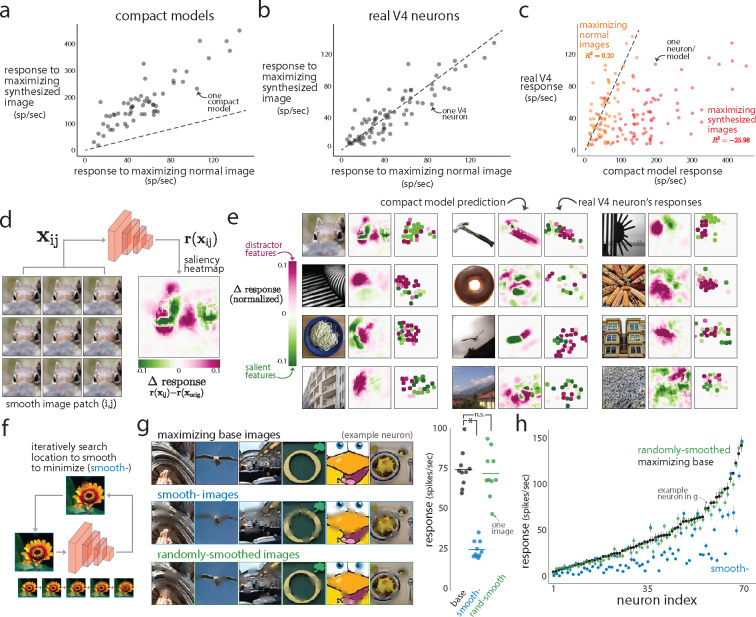
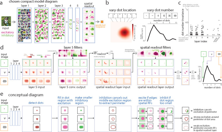
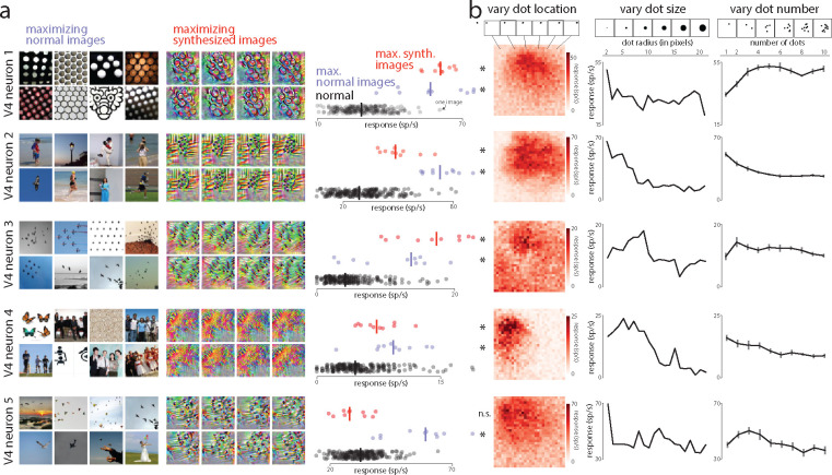
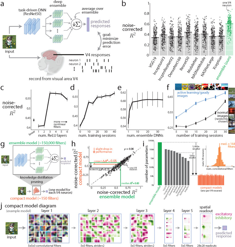
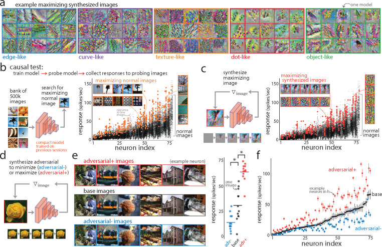
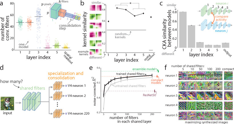
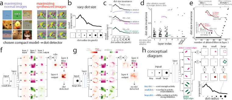
A powerful approach to understanding the computations carried out in visual cortex is to develop models that predict neural responses to arbitrary images. Deep neural network (DNN) models have worked remarkably well at predicting neural responses [1, 2, 3], yet their underlying computations remain buried in millions of parameters. Have we simply replaced one complicated system in vivo with another in silico? Here, we train a data-driven deep ensemble model that predicts macaque V4 responses ~50% more accurately than currently-used task-driven DNN models. We then compress this deep ensemble to identify compact models that have 5,000x fewer parameters yet equivalent accuracy as the deep ensemble. We verified that the stimulus preferences of the compact models matched those of the real V4 neurons by measuring V4 responses to both 'maximizing' and adversarial images generated using compact models. We then analyzed the inner workings of the compact models and discovered a common circuit motif: Compact models share a similar set of filters in early stages of processing but then specialize by heavily consolidating this shared representation with a precise readout. This suggests that a V4 neuron's stimulus preference is determined entirely by its consolidation step. To demonstrate this, we investigated the compression step of a dot-detecting compact model and found a set of simple computations that may be carried out by dot-selective V4 neurons. Overall, our work demonstrates that the DNN models currently used in computational neuroscience are needlessly large; our approach provides a new way forward for obtaining explainable, high-accuracy models of visual cortical neurons.

Extended Data Figure 1:. Detailed diagrams of deep ensemble model and compact model network architectures.

a. Detailed diagram of our deep ensemble model, which uses the early layers of a task-driven ResNet50 and an ensemble of ResNet-like DNNs. Each ensemble DNN has skip-connection blocks and relies on separable convolutions to reduce the number of parameters. The shapes of each output activity tensor as well as the shapes of the weight tensors are in parentheses nearby their corresponding layer. See Methods for details. b. Diagrams of linear mappings between a model’s embedding output activity $X$ (of shape $p\times p\times k$ for $p$ downsampled pixels and $k$ channels/filters) and V4 responses. Ridge regression fits a weight matrix ${\beta }^{\text{ridge}}$ of shape $p\times p\times k$ with $L_2$ regularization (top). The predicted response $\hat{r}$ is computed from embedding $X$ as the following: $$\hat{r}=\sum _k\sum _{i,j}{\beta }_{ijk}^{\text{ridge}}{X}_{ijk}+{\beta }_0$$ where ${\beta }_0$ is an offset term. The factorized linear mapping [110] fits two weight matrices: a mixing matrix ${\beta }^{\text{mixing}}$ of shape $k\times 1$ that integrates or “mixes” information across filters and a spatial pooling matrix ${\beta }_{\text{spatial}}$ of shape $p\times p$ that integrates spatial information. The predicted response $\hat{r}$ is computed as the following: $$\hat{r}=\sum _k{\beta }_k^{\text{mixing}}\sum _{i,j}{\beta }_{ij}^{\text{spatial}}{X}_{ijk}+{\beta }_0$$ This factorized mapping can be thought of as a low-rank approximation to ridge regression. Comparing the number of parameters between the two mappings reveals that the number of parameters of ridge regression $(p\cdot p\cdot k)$ is substantially greater than that of the factorized linear mapping $(p\cdot p+k)$. Given that the linear mapping needs to be fit to a small amount of training data (typically < 1,500 images), the factorized linear mapping will less likely overfit due to its smaller number of parameters (Ext. Data Fig. 2). c. Although the recording electrode array was chronically implanted, we could not be entirely certain that we recorded the same V4 neuron across two or more sessions. Thus, we assumed that each recording session was a new sampling of V4 neurons (with the caveat that some neurons were likely present in multiple sessions). To build this assumption into the model, we gave each recording session its own linear mapping between the embedding output of the deep ensemble model and that session’s V4 responses (${\beta }_1,{\beta }_2,\dots ,{\beta }_N$ for $N$ sessions). When training the deep ensemble model on the $i$th session, we set the weights of β to 0 (but kept all other weights of the deep ensemble the same) and performed stochastic gradient descent end-to-end; we found that resetting $\beta$ with previously-trained $\beta$’s led to overfitting and worse performance. To evaluate the model’s predictions on a held out session, we trained $\beta$ on a portion of the image/response pairs and predicted the remaining pairs in a cross-validated manner. d. Detailed diagram of a compact model, including the separable convolutional layers, batchnorms, and ReLUs. The $i$th layer has its own number of filters $K_i$ except for layers 1 and 2 which have the same number of filters $\left(K_1=K_2\right)$ due to layer 1 being fully convolutional. We illustrate separable convolutions in two parts: the convolutional filters (red squares) and the mixing weights (green matrices). Each convolutional filter processes the activity map of one input filter, making the number of convolutional filters in the $\ell$th layer equal to $K_{\ell -1}$, the number of output channels for the $(\ell -1)$th layer. Each mixing matrix linearly combines the output of these convolutional filters across filters and takes shape $K_{\ell -1}\times K_{\ell }$. Layer 1 is a fully convolutional layer, and the spatial readout layer is a dense layer but can be thought of as a set of spatial receptive fields whose output is summed together. See Methods for further details.

Extended Data Figure 2:. Comparing our noise-corrected R2 values versus those reported in a previous study.

Comparing noise-corrected $R^2$s across studies can be difficult, as they often differ in spike sorting procedures, the types and numbers of images presented, how the noise-corrected $R^2$ metric is computed, and how DNN features are mapped to V4 responses. Indeed, for linearly mapping task-driven DNN features to V4 responses, we find a difference between our reported noise-corrected $R^2=0.45$ (Fig. 1b) with another reported noise-corrected $R^2=0.89$ from a previous study [40]. Here, we determine that this difference is primarily due to different noise-corrected $R^2$ metrics and spike sorting criteria. a. A key difference between our study and [40] is our noise-corrected $R^2$ metric. [40] use the BrainScore $R^2$, which computes an $R^2$ ceiling by splitting repeats into two halves, corrected with the Spearman-Brown procedure [30]. The BrainScore $R^2$ is computed with the following pseudocode: We use a recently-proposed unbiased noise-corrected $R^2$ metric (mathematically defined in Methods), which was shown to be more consistent at estimating the true $R^2$ versus other proposed $R^2$ metrics [106]. For each of our 219 recorded neurons on 4 held out sessions, we computed the unbiased $R^2$ versus the BrainScore $R^2$ using a linear mapping (ridge regression) between ResNet50 features and V4 responses (cross-validated). We noticed a sizable increase of the BrainScore $R^2$ (dots to the right of dashed line, $\mathrm{\Delta }{R}^2\approx 0.15$), including some neurons with BrainScore $R^2>1$ (dots to the right of 1), likely caused by too few repeats to properly estimate $R^2$. This overestimation in $R^2$ was expected and motivation for an unbiased $R^2$ [31]. This increase appeared to be a shift for every neuron, as the unbiased $R^2$ was correlated with the BrainScore $R^2$ across neurons $(\rho =0.84)$. Each dot denotes a V4 neuron; $\mu$ denotes the mean $R^2$ across neurons. b. Because [40] uses the BrainScore metric, we wondered if this entirely explained the difference between the reported $R^2$s. We re-computed the BrainScore and unbiased $R^2$ metrics for the publicly-available V4 responses from [40] with ResNet50 features and found a similar difference in mean noise-corrected $R^2$ with a larger BrainScore $R^2$ (dots to the right of dashed line, $\mathrm{\Delta }{R}^2\approx 0.15$). Again, this increase appeared to be a shift, as the $R^2$s were correlated across neurons $(\rho =0.86)$. We note that our reported BrainScore $R^2=0.73$ was lower than that reported by [40] $\left(R^2=0.89\right)$ for the same data. To account for this difference, we trained a factorized linear mapping [110] (same as used in [40]) and achieved a BrainScore $R^2=0.83$; we suspect using their retinal transformation would then achieve the same BrainScore $R^2$. We conclude that the BrainScore $R^2$ metric adds ~0.15 to an unbiased $R^2$ metric; however, for the same unbiased $R^2$ metric, we see a difference of $\mathrm{\Delta }{R}^2\approx 0.2$ (compare orange $\mu$ between a and b; similar for BrainScore $R^2$). Thus, a difference in metric contributes to differences in reported $R^2$s but does not provide a full explanation. c. We checked another possibility—in our study, we presented colorful natural images while [40] presented grayscale images with foreground objects placed on unrelated natural backgrounds (see inset images). To see if this difference in image type could lead to differences in $R^2$, we used one recording session to present 600 colorful natural images and 600 images from [40]. We found that when predicting these V4 responses with ResNet50 features, there was only a modest increase in $R^2$ for the grayscale images (mean $R^2=0.32$ for grayscale images versus mean $R^2=0.28$ for colorful images). We also observed that these $R^2$s were correlated across neurons $(\rho =0.39)$. Thus, the differences in image statistics likely was not a contributing factor in the differences in unbiased $R^2$ between our responses and responses in [40]. We conclude that this difference in $R^2$ arises because of differences in spike sorting and electrode unit criteria. [40] have stricter criteria for retaining recorded units (neurons must be present across multiple sessions, single-unit isolation, etc.), whereas our criteria are less strict (neurons need only be present for one session, multi-unit activity is possible). This highlights the need to test one’s model on multiple data sets from different laboratories [30]. d-e. Compared to a task-driven DNN model that appears to generalize well for any V4 neuron, we tailored our data-driven deep ensemble model to predict only our recorded V4 responses. It was unclear if our deep ensemble model could generalize to V4 neurons on which it was not trained (i.e., generalize to “out-of-distribution” V4 neurons). To test this, we sought to use the deep ensemble model to predict the V4 responses from [40]. To make a fair comparison, we recorded V4 responses to images from [40]; we confirmed that our deep ensemble model predicted responses to these images (d, median unbiased noise-corrected $R^2\mathrm{m}=0.61$) to the same extent as those to natural images (Fig.1b, median $R^2\mathrm{m}=0.61$). Similarly, using ResNet50 features had nearly identical prediction performances (d, median unbiased $R^2\mathrm{m}=0.43$; Fig. 1b, median $R^2\mathrm{m}=0.43$). This suggests that our deep ensemble model could predict our V4 responses to images from [40] to the same extent as those to colorful natural images, consistent with ResNet50’s predictions (c). Next, we performed the same analysis but for V4 responses from [40]. Using ResNet50 features increased prediction performance (d, $\mathrm{m}=0.43$ to e, $\mathrm{m}=0.60$), consistent with the increased prediction performance between our V4 responses to colorful natural images (a, orange, $\mu =0.41$) and V4 responses from [40] (b, orange, $\mu =0.59$). We expected prediction performance for the deep ensemble to worsen between our V4 responses and responses from [40], as our deep ensemble model was optimized only for our recorded V4 responses. However, this was not the case: Prediction performance remained at the same level between the two (d, $\mathrm{m}=0.61$ versus e, $\mathrm{m}=0.62$). This suggests that our deep ensemble model can generalize to new V4 neurons, although we lose the performance gains from training on these V4 neurons. We expect that as our deep ensemble model is trained on responses from more V4 neurons, its generalization ability will increase, surpassing that of ResNet50. f-g. For completeness, we also consider a newly proposed mapping between DNN features and V4 responses that factorizes a linear mapping into a ‘spatial’ stage and a channel ‘mixing’ stage [110] (see Methods). We found a modest increase in prediction performance for this factorized linear mapping versus a linear mapping identified with ridge regression, both when using ResNet50 features (f, median unbiased $R^2\mathrm{m}=0.46$ versus $\mathrm{m}=0.43$) and the output embeddings of the deep ensemble model (g, median unbiased $R^2\mathrm{m}=0.61$ versus $\mathrm{m}=0.59$) for V4 responses to natural images in our 4 held out recording sessions. We suspect that this increase, smaller than those observed previously [40, 110], arises because we have roughly double the number of images shown per session on which to train and test the mappings. h. We designed a procedure to prune filters that, if ablated, led to little change in the model’s output. Our pruning procedure starts with filters in the deepest layers and proceeds backwards to filters in the earliest layers. After pruning, we found the earliest layers had larger numbers of filters (~50 filters each, Fig. 3a) than the deepest layers (5–10 filters each, Fig. 3a). However, we wondered if this trend arose because we pruned filters in the deepest layer first. To test for this, we reversed the order of pruning to begin with the earliest layer (i.e., layer 1) and continue to the deeper layers. This reversal led to a larger number of filters overall (median number of filters across neurons was 264 filters versus the 164 filters in the deep-to-early-layer pruning), yet we still found the same trend of a larger number of filters in early versus deeper layers (compare h with Fig. 3a). We conclude that the consolidation step identified in our compact models was not due to the way in which the model was pruned.

Extended Data Figure 3:. Maximizing synthesized images for all compact models.

For each compact model, we computed the maximizing synthesized image via gradent ascent techniques (Fig. 2a). Here, we show these images for all compact models (one image per compact model). For visual clarity, we loosely grouped images into categories by eye. We make no claims about grouping in V4 neurons; in fact, the mean signal correlation squared across all pairs of compact models was low (${\rho }^2=0.11$ between model responses to 10,000 normal images). This remained true when controlling for spatial receptive field location (Fig. 3c, layer 5). Thus, the stimulus preferences across V4 neurons appear to be largely heterogeneous, allowing for a highly-expressive set of features for downstream processing (e.g., IT neurons).

Extended Data Figure 4:. Further causal tests of the compact models.

Our compact models’ predictions held up to causal testing (Fig. 2), including identifying maximizing normal and synthesized images. Here, we compare which type of these images better drives V4 responses. In addition, we present results of further causal tests, including identifying saliency maps and “adversarial smooth” images. a-c. We found that the compact models predicted much stronger V4 responses to maximizing synthesized images versus maximizing (normal) images (a, dots above dashed line; difference of means between maximizing synthesized and maximizing normal: 111.7 spikes/sec, $p<0.002$, permutation test). However, this was not the case for the real responses—both types of images evoked similarly large responses (b, dots hug dashed line, difference of means not significant, $p=0.836$, permutation test). This difference largely stems from the compact models’ inability to predict V4 responses to maximizing synthesized images (c, red dots, coefficient of determination $R^2=-26.0$, not noise-corrected) whereas their prediction for maximizing normal images remains relatively intact (c, orange dots, coefficient of determination $R^2=0.2$, not noise-corrected). Each dot denotes a neuron’s response, averaged over repeats and maximizing images (if multiple maximizing images were shown for a V4 neuron, see Fig. 2b and c). This inability to predict maximizing synthesized images was not unexpected—the optimizing procedure had full access to every weight and every pixel to optimize an image customized for that compact model. Moreover, the resulting synthesized images were well outside the distribution of training images, and we would expect poor prediction for these outlying regions of image space. This was one motivation for training our deep ensemble model with closed-loop active learning (Fig. 1f) in which we trained the model on out-of-distribution images. We were also suprised that the maximizing normal images evoked V4 responses as large as those to maximizing synthesized images (b). This suggests that one cannot rule out choosing from a large pool of candidate images (in this case, 500,000 candidate images) to maximally drive V4 responses. d. A commonly-used approach to explain a DNN’s output is to identify which parts of an input image are the most-relevant or “salient” for the DNN’s prediction; this approach is called saliency analysis [123]. One implementation is to smooth a small patch of the image (small orange circles in example images denote smoothed patches; these circles were not present in actual stimuli) and see if the resulting response is larger or smaller than the response to the original image. An increase in response (pink) indicates that the visual feature within the smoothed patch is distracting, as removing this feature leads to a larger response. Likewise, a decrease in response (green) indicates a salient or excitatory visual feature. We passed as input a set of images where the $(i,j)$th image had a smoothed image patch centered at $(i,j)$. We then formed a heatmap of the resulting responses $\mathbf{r}$ based on the $(i,j)$ of the image patch (‘saliency heatmap’). For this example image of a squirrel and the chosen compact model, the most salient features are the eyes (green regions), while the most distracting features are the fur texture and the edges around the left eye (pink regions). e. In our causal experiments, we probed the trained compact models to identify maximizing normal images(Fig. 2b). For each maximizing normal image, we computed the saliency heatmap of the compact model (‘compact model prediction’) following the procedure in d. We then used these predictions to smooth 25 non-overlapping image patches that led to the largest changes in responses (where the number 25 was chosen as a compromise between covering as much as the image as possible within recording time constraints). On a following session, we showed each ‘base’ image as well as the 25 images, each with one smoothed image patch. For each example image shown here, we matched a V4 neuron with the image’s corresponding compact model (in the same way as in Fig. 2) and computed the resulting saliency heatmap for V4 neurons (rightmost panels). Responses were z-scored using the mean and standard deviation estimated with the V4 neuron’s responses to all normal images shown in the session. We found that V4 neurons did vary their responses to local smoothing and that these changes in responses largely matched those predicted by the compact models. Thus, for a given image, a V4 neuron’s response can be suppressed and excited by different local visual features; our compact models can be used to predict which features at which locations. f. Inspired by the saliency approach in d and e, we causally tested our compact models by having them predict which visual features of an image to smooth in order to minimize a V4 neuron’s response. We first began with the compact model’s maximizing normal image as a base image. Then, in a greedy manner, we iteratively chose an image patch to smooth that led to the smallest response as predicted by the compact model (‘smooth−’, see orange circle). Successive iterations added image patches that did not overlap with previously-chosen image patches. This led to an image with specific visual features smoothed away. Bottom inset: a sequence of images for which a base image is cumulatively smoothed at different patches determined by the compact model’s predictions; the final smoothed image is the rightmost. g. Example base images (left, top row, ‘maximizing base images’), smoothed versions to minimize the model-output response as predicted by a compact model (left, middle row, ‘smooth− images’), and images for which randomly-chosen patches were smoothed as a control (left, bottom row, ‘randomly-smoothed images’). The randomly-smoothed and smooth− images had the same number of pixels smoothed. These example maximizing base images and randomly-smoothed images elicited similarly large responses from a V4 neuron (right, black versus green dots, $p=0.70$, permutation test) whereas the smooth− image led to a substantially smaller response (black versus blue dots, $p<0.002$, permutation test, asterisk). Each dot denotes the repeat-averaged response to one image. h. Responses for all V4 neurons from two recording sessions (each session from a different animal). V4 neurons were matched to compact models via held out images (same procedure as used in Fig. 2b–f). For one session, only one base image was shown per compact model; for these images, dots denote repeat-averaged responses with no error bars. For the other session, we presented 10 base images (and their smooth− and randomly-smoothed counterparts) per neuron. For this session, dots denote the average response over the 10 images (and their repeats), and error bars denote s.e.m. over the 10 images. Neurons were sorted based on mean response to the base images. We found that responses to smooth− images were roughly half as small as responses to the base images across V4 neurons (blue versus black dots, normalized percent change computed as $\mathrm{\%}\mathrm{\Delta }\bar{r}=100\cdot [\bar{r}(\mathrm{s}\mathrm{m}\mathrm{o}\mathrm{o}\mathrm{t}\mathrm{h}-)-\bar{r}(\mathrm{b}\mathrm{a}\mathrm{s}\mathrm{e})]/\bar{r}\left(\mathrm{b}\mathrm{a}\mathrm{s}\mathrm{e}\right)$: mean $\mathrm{\%}\mathrm{\Delta }\bar{r}\pm \mathrm{s}.\mathrm{e}.:-46.1\mathrm{\%}\pm 3.5\mathrm{\%}$). Little to no decrease between maximizing base and randomly-smoothed images (green versus black dots, mean $\mathrm{\%}\mathrm{\Delta }\bar{r}\pm \mathrm{s}.\mathrm{e}.:-3.7\mathrm{\%}\pm 1.9\mathrm{\%}$). Thus, in a causal test, the compact models accurately predicted which visual features (and their spatial information) were most salient to the V4 neurons. This provides further evidence that the compact models accurately capture the stimulus preferences of V4 neurons—and what visual features in those preferred stimuli are most important to the V4 neuron.

Extended Data Figure 5:. Explaining a dot-detecting compact model’s selectivity for multiple dots.

To understand the computations within a compact model, we chose to investigate a particular compact model that resembled a dot detector (Fig. 4). We focused on the model’s selectivity to dot size (Fig. 4b) and uncovered a simple computation by isolating the filters that contributed to dot size selectivity (Fig. 4c–h). However, we suspected this compact model was also selective to the number of dots, as its preferred stimuli typically had two to five dots in the image (Fig. 4a). Here, we investigate this model’s dot number selectivity. a. Diagram of the compact model that resembles a dot detector. We expected to see dot-like filters (i.e., middle excitation surrounded by inhibition or vice versa) in layers 1–3 but found none. This led us to identify corner and large edge detecting filters that ultimately contributed to dot size selectivity (Fig. 4c–h). b. Besides varying dot size, we also varied the location of a small dot with a radius of 5 pixels (left, ‘vary dot location’) and dot number (right, ‘vary dot number’). The compact model (same as in a and Fig. 4) preferred three dots to the center right (with dot radii of 5 pixels, from Fig. 4b). Given this compact model’s preferred stimuli (Fig. 4a) and selectivity to dot location (left), dot number (right), and dot size (Fig. 4b), we conclude that this compact model is a dot detector. c. In the same manner as we identified filters contributing to dot size selectivity (Fig. 4c and d), we ablated each filter and measured the model’s dot number invariance. A dot number invariance of 1 indicates that after ablating a filter, the model is no longer able to detect different numbers of dots; a dot number invariance of 0 indicates no change in the model’s output (i.e., dot number selectivity remains intact). We found that none of the filters contributed strongly to dot number selectivity (i.e., no filter, once ablated, led to a large increase in dot number invariance); this differs from the highly contributing filters for dot size selectivity (compare c with Fig. 4d, filters with DSI > 0.75). This indicates that dot number selectivity emerges from the last spatial readout layer. d. To understand the specific computations of dot number selectivity, we passed in three input images with different numbers of dots (‘input image’). We then observed the resulting activity and filter weights for layer 5 and the spatial readout layer. We noticed that the input to layer 5 (‘layer 5 input’) appeared to detect the presence of a dot at any given location (matching our intuition for identifying a single dot in Fig. 4f–h). The layer 5 filters (chosen as those with the largest dot number invariance in c) appeared to extract specific patterns of the detected dots: After convolution, some filters formed large excitatory regions around the dots whereas others formed smaller regions of inhibition (‘layer 5 conv. output’). After passing through a linear combination of its filters (by multiplying with readout matrix $W_{\text{readout}}$) and the ReLU activation function, we found that most of the dot regions were extinguished with some filters activated by the edges or shells of the dot region (‘spatial readout layer input’). This activity was then excited or suppressed by spatial readout filters that act as spatial receptive fields. After taking a linear combination over filters (‘sum over filters’), we observed that a single small dot had both excitation and inhibition (top activity map), while three dots led to large activity around the region of the dots (middle activity map). Many dots led to little to no activity (bottom activity map). Summing over spatial information (i.e., pixels) recreated the selectivity to dot number (rightmost plot). We illustrate the circuit mechanisms in d with a conceptual diagram. The key concept is that the model identifies a region of dots, extracts the shell around this region (by creating a larger excitatory region and a smaller inhibitory region), and queries the size of this shell. Too small a region (i.e., a single dot) leads to weak activity and inhibition (rightmost, top activity map). Too large a region leads to weak excitation, as the shell of the region is outside the spatial receptive field. Only an appropriately sized region (i.e., a certain number of dots) will fit within the spatial receptive field, leading to strong excitation. This results suggest that a key computation in dot number selectivity is to extract “regions” of interest and then to identify the edges of these regions. If the number of dots is too large, the region’s edge will be outside the spatial receptive field, yielding a small response. This may be a reoccurring theme in the visual cortex for other visual features.

Extended Data Figure 6:. Identifying real V4 dot detectors with causal tests.

To confirm the presence of dot-detecting V4 neurons, we ran causal tests specifically tailored for compact models that resemble dot detectors. We first identified compact models by training on previous recording sessions. From the identified compact models, we chose 5 compact models that most resembled dot detectors based on their stimulus preferences (i.e., maximizing normal and synthesized images) and their responses to artificial dot stimuli (see Fig. 4a and b and Ext. Data Fig. 5). We note that the chosen dot detecting compact model in Figure 4 was not one of the chosen, as this compact model matched to a V4 neuron from another animal. For a future recording session, we presented the maximizing normal and synthesized images of the 5 chosen models as well as artificial dot stimuli (same dot stimuli as in Fig. 4b and Ext. Data Fig. 5b). We identified the 5 recorded V4 neurons that best matched the predictions of the 5 compact models (by computing the noise-corrected $R^2$ from all other images shown in the session, same procedure as in Fig. 2b–f) and show their responses here. a. The maximizing normal images (left, examples) and maximizing synthesized images (middle, examples) chosen from the 5 compact models tended to more strongly drive V4 responses than responses to normal images (right, ‘max. synth. images’ and ‘max. images’ dots more to the right than ‘normal’ black dots). Each dot is the repeat-averaged response to one image; lines denote medians. All maximizing stimuli yielded median responses significantly greater than the median response to normal images ($p<0.02$, one-sided permutation test, asterisks) except one set of maximizing synthesized stimuli (bottom row, V4 neuron 5, red dots, $p=0.922$, one-sided permutation test). This failure could be from instability in the electrode array (i.e., the V4 neuron on which the compact model was trained no longer was accessible by the electrode array) or due to model mismatch. b. V4 responses to the artificial dot stimuli that varied in dot location (left), dot size (middle) and number of dots(right). Same format as in Figure 4b and Extended Data Figure 5. Dot locations were subsampled to 28 × 28 locations to limit the number of images. Error bars in ‘vary dot number’ denote 1 s.e.m. across 10 different images, where each image had the same number of dots but in different locations randomly chosen to be nearby the preferred location (see Methods). We found that these V4 neurons had preferred dot locations (b, left), preferred dot sizes (b, middle), and preferred numbers of dots (b, right), consistent with these V4 neurons being dot detectors. Thus, these results confirm the presence of dot detectors in V4. We observed diverse selectivity to dot size, including V4 neurons selective to the tiniest dots (neurons 1, 2, and 5) and small dots (neurons 3 and 4). Similarly, we observed selectivity to one dot (neurons 2 and 4), 2 dots (neuron 3), and 3 or more dots (neurons 1 and 5). Thus, even within the class of dot detectors, there appears to be large diversity in stimulus preferences.

Extended Data Figure 7:. Example visual stimuli shown in experiments.

Example images for each type of visual stimuli shown in our experiments. Example images were randomly selected for each type. See Methods for details about how images were chosen or generated.

Figure 1:. Identifying compact models of macaque V4 neurons.

a. We presented natural images while recording from neurons in visual cortical area V4. We model the mapping between images and repeat-averaged V4 responses (spike counts taken in 100 ms bins) with a two-stage model. The first stage is to pass the image through the early and middle layers of a task-driven DNN trained to perform object recognition (blue, ResNet50). We then take the output activity of a middle layer of ResNet50 as input to the second stage—an ensemble of convolutional DNNs (green). Each ensemble DNN has the same architecture but different random initializations. The weights of the deep ensemble are shared across recording sessions, but we assume a new set of neurons each session by fitting new linear mappings between the deep ensemble’s output and V4 responses for each session. The final predicted V4 responses are the outputs of these linear mappings averaged across the ensemble (see Ext. Data Fig. 1 for detailed diagrams). b. Comparison of prediction performance for different DNN models on held-out images and recording sessions. DNN models included task-driven models (black) as well as our proposed data-driven deep ensemble model (green). We report noise-corrected $R^2$, which accounts for repeat-to-repeat noise in the estimates of the repeat-averaged responses (Ext. Data Fig. 2). Each dot denotes one V4 neuron. c-f. Four modeling improvements that boosted prediction performance. These included placing a nonlinear mapping between ResNet50 features and V4 responses (c), training on a large number of recording sessions (d), using a deep ensemble with many small DNNs (e), and training on images chosen adaptively by active learning and gaudy images versus randomly-chosen normal images (f). See Methods for details on each analysis. Lines denote medians, error bars denote 90% bootstrapped confidence intervals. g. Framework to identify compact models. We take our large deep ensemble model (top) and use the model compression techniques (knowledge distillation and pruning) to identify a compact model, one for each V4 neuron (bottom). h. Prediction performance on held-out V4 responses for the deep ensemble model versus that of the compact models. Each dot denotes one V4 neuron; the dashed line denotes the same level of prediction. On average, the compact models predicted V4 responses only slightly worse than the deep ensemble model with a decrease in median noise-corrected $\mathrm{\Delta }{R}^2=0.05$ (orange line), much smaller than that of task-driven ResNet50 features ($\mathrm{\Delta }{R}^2=0.15$, black line). The $R^2$s between compact and ensemble model predictions across neurons were highly correlated ($\rho =0.96$), suggesting that no group of V4 neurons (e.g., “dot detectors”) was more poorly explained than another group by the compact models. i. Number of parameters (including linear mappings) for our deep ensemble model (green), task-driven models (black), and compact models (orange). The y-axis is in log-scale. Inset: Total number of convolutional filters for each compact model across V4 neurons; the median was 164 filters, whereas our deep ensemble model had ~150,000 filters. j. Diagram for an example compact model showing all weight parameters for its convolutional filters. Pink denotes positive (or excitatory) weights, and green denotes negative (or inhibitory) weights. Because layer 1 filters directly take the RGB image as input, the weights are colored based on RGB channels. For clarity, the mixing weights and batchnorm weights are not shown (see Ext. Data Fig. 1).

Figure 2:. Causally testing the predictions of compact models.

a. Preferred synthetic stimuli of selected compact models (one stimulus per model; see Ext. Data Fig. 3 for all compact models). Each image is optimized via gradient ascent to maximize a model’s output response (see Methods). For illustrative purposes, preferred stimuli were loosely placed by eye into categories (e.g., “edge-like” detectors, “curve-like” detectors, etc.). b. Causal test in which we trained a compact model on previous recording sessions, probed the model to identify images from a bank of 500,000 candidate images that maximize the model’s output (left), and then recorded V4 responses to these maximizing normal images in future sessions (right). The maximizing normal images drove larger V4 responses (orange dots, normalized percent change computed as $\mathrm{\%}\mathrm{\Delta }\bar{r}=100\cdot \left(\bar{r}\right(\mathrm{m}\mathrm{a}\mathrm{x})-\bar{r}(\mathrm{n}\mathrm{o}\mathrm{r}\mathrm{m}\mathrm{a}\mathrm{l}\left)\right)/\bar{r}\left(\mathrm{n}\mathrm{o}\mathrm{r}\mathrm{m}\mathrm{a}\mathrm{l}\right)$: mean $\mathrm{\%}\mathrm{\Delta }\bar{r}\pm \mathrm{s}.\mathrm{e}.:137.3\mathrm{\%}\pm 9.2\mathrm{\%}$, where $\bar{r}$ is the mean response over images) than responses to randomly-chosen normal images (black dots). Each dot denotes the repeat-averaged response to one image. Each neuron index (x-axis) refers to one of the 78 neurons recorded from two monkeys, ordered by average response to the normal images. Insets show maximizing normal images for three example neurons. c. Causal test for maximizing synthesized images of the compact models. Each synthesized image started as a white noise image and iteratively changed via gradient ascent by propagating the gradient with respect to the model’s output back through the compact model (example iterations shown in bottom left inset). In future recording sessions, the maximizing synthesized images elicited larger V4 responses (red dots, $\mathrm{\%}\mathrm{\Delta }\bar{r}=152.8\mathrm{\%}\pm 10.8\mathrm{\%}$) than responses to randomly-chosen normal images (black dots). Insets show the maximizing synthesized images for three example neurons (same as in b). d. Causal test for adversarial images of the compact models. We define an adversarial image as a slight perturbation to some base image that yields a large change in the model’s output. Adversarial images were synthesized via gradient descent to minimize the model’s output (‘adversarial−’) or gradient ascent to maximize the model’s output (‘adversarial+’). Synthesis stopped when differences in pixel intensities between the base image and the adversarial image passed a threshold. e. Example adversarial+, base, and adversarial− images for an example compact model (left). As predicted by the compact model, a corresponding real V4 neuron responded less to the adversarial− images (blue dots) and more to the adversarial+ images (red dots) compared to responses to the base images (black dots). Each dot denotes the repeat-averaged response to one image; lines denote means, and asterisks denote $p<0.05$ (permutation test). f. In future recording sessions, adversarial+ images drove larger responses (red dots, $\mathrm{\%}\mathrm{\Delta }\bar{r}=83.6\mathrm{\%}\pm 5.9\mathrm{\%}$) and adversarial− images drove smaller responses (blue dots, $\mathrm{\%}\mathrm{\Delta }\bar{r}=-33.2\mathrm{\%}\pm 2.5\mathrm{\%}$) compared to responses to base images (black dots). Dots denote means, and error bars denote 1 s.e.m. across 10 or more base images per neuron.

Figure 3:. Compact models share similar filters in early layers but then heavily specialize via a consolidation step.

a. Number of convolutional filters per layer as determined by our model compression framework; each layer potentially has up to 100 filters. Each dot denotes one compact model; lines denote medians. Layers 1 and 2 have the same number of convolutional filters as defined by the compact model’s architecture. Inset: diagram depicting activity map shapes ($p\times p\times k$ for $p$ pixels and $k$ filters) for each layer. b. Kernel similarity between kernel weights of convolutional filters from the same layer across compact models. A kernel similarity close to 1 indicates that any convolutional filter from a given layer will have a closely matching filter (i.e., matching in its kernel weight pattern) from the same layer. For reference, we assessed the kernel similarity for filters whose weights are drawn randomly from a standard normal distribution (gray). Because layer 1 weights were not smoothed during training and the spatial readout filters were much larger (28×28 pixels vs. 5×5 pixels), it was not fair to compare the kernel similarities of these layers to the other remaining layers (layers 2–4). Layers 2 and 3 had a significantly higher mean kernel similarity than that of layers 4 and 5 ($p<0.002$, permutation test). Dots denote mean, and error bars denote 1 s.d. across 500 runs of sampling pairs of models (see Methods). c. Centered kernel alignment (CKA) similarity between the activity of the same layer for two compact models. The activity is the output of each layer’s filters for 10,000 normal images. A CKA similarity close to 1 indicates that the two layers have near identicial representations up to a rotation. Layers 1 and 2 had significantly higher CKA similarity than that of layers 3 and 4 ($p<0.002$, permutation test). The error bars denoting 1 s.e.m. are small due to the large number of pairs of models (~23,000 pairs). d. Diagram of a ‘shared’ compact model to predict all V4 neurons together. The model constrains each V4 neuron to use the same shared filters in the first 3 layers (i.e., early layers), while the remaining 3 layers allow for consolidation and specialization (see Methods). It is unknown how many shared filters in the early layers are needed to explain V4 responses. e. Prediction performance of V4 responses while varying the number of shared filters in the early layers. For each number, a new compact model was trained via distillation by using the responses of the ensemble model (‘trained shared filters’); pruning was not performed. Fixing the kernel weights of the early layers to their initial random values (but allowing all other parameters in the early layers to be trained) led to worse prediction performance (gray line below black line). For reference, we re-computed performance for the ResNet50 features, the compact models, and the deep ensemble model (bottom, middle, and top dashed lines, respectively). Dots denote means; error bars denote 1 s.e.m. f. Maximizing synthesized images of the shared compact model with different numbers of shared filters (columns) as well as individual compact models (rightmost column) for five example V4 neurons.

Figure 4:. Uncovering the internal computations of a dot-detecting compact model.

a. Preferred stimuli (maximizing normal and synthesized images) for a compact model chosen for its resemblance to a dot detector. These preferred stimuli drove large model responses well beyond the response range for normal images. b. For the chosen compact model in a, model responses to artificial dot stimuli in which we varied the size of a dot centered in the preferred location of the model. The compact model was also selective to dot location and dot number (Ext. Data Fig. 5). c. Responses from the model for either no ablation (black lines) or ablated filters (color lines) to artificial stimuli varying in dot size. An ablated filter (‘L4F1’ stands for Layer 4, Filter 1) has its kernel weights set to 0. We measured each filter’s dot size invariance (DSI) as the extent to which responses change due to ablation (i.e., the change between black and color lines, see Methods). A DSI = 1 indicates that, after filter ablation, the model is invariant to dot size (top panel, blue line is flat)—in other words, that filter is necessary for the model’s dot selectivity. d. Dot size invariance for each individual convolutional filter in the chosen compact model. Color dots correspond to example filters in c. e. Cumulatively ablating filters in layer 3 to identify the subset of filters that strongly contribute to dot selectivity. To do this, we keep ablating filters until DSI = 1 (i.e., until we observe a substantial change in the model’s responses). For each iteration, we choose a filter from the remaining filters that, once ablated, increases DSI the least. Little to no increase in DSI indicates that the ablated filter weakly contributes to dot selectivity (leftmost dots); a large increase indicates a strong contribution to dot selectivity (rightmost dots). f. Investigating the layer 3 filters that strongly contribute to dot selectivity (i.e., 6 of the 12 rightmost dots in e). We pass as input an image with a small dot at the compact model’s preferred location (‘small dot’). The input activity map for each layer 3 filter (‘layer 3 input’) represents the processed image after the first two layers; each activity map is then convolved by its corresponding layer 3 filter (‘layer 3 filters’) to produce the convolved output (‘layer 3 conv. output’). This convolved activity is then summed element-wise across filters, passed through a ReLU, and then convolved again by a layer 4 filter to produce the processed output activity (‘layer 4 output’). In this case of a small dot, the output activity is large (dark red), indicating the presence of a dot (‘dot detected’). For clarity, the activity maps were cropped around the dot’s location; activity outside this cropped region was a constant value. g. Analyzing the same filters as in f except for an input image with a large dot (‘large dot’). In this case, the output activity (‘layer 4 output’) is small (light red), indicating that no dot is present (‘no dot detected’). h. Illustrative diagram describing the computations in the dot detector compact model. The 4 excitatory filters (pink) detect the 4 corner edges of the dot while the 2 inhibitory neurons (green) detect large edges. For a tiny dot (‘tiny’), the excitatory activity is weak, leading to a weak response. For a small dot (‘small’), the strong excitatory activity overlaps when summed (producing an even larger response) while inhibition is weak, leading to an overall large response. For a large dot (‘large’), the excitatory activity is strong but does not overlap; in addition, inhibition is strong. This leads to an overall weak response.

References

1. Yamins Daniel LK and DiCarlo James J. Using goal-driven deep learning models to understand sensory cortex. Nature Neuroscience, 19(3):356–365, 2016. - PubMed
1. Richards Blake A, Lillicrap Timothy P, Beaudoin Philippe, Bengio Yoshua, Bogacz Rafal, Christensen Amelia, Clopath Claudia, Costa Rui Ponte, Berker Archy de, Ganguli Surya, et al. A deep learning framework for neuroscience. Nature neuroscience, 22(11):1761–1770, 2019. - PMC - PubMed
1. Doerig Adrien, Sommers Rowan P, Seeliger Katja, Richards Blake, Ismael Jenann, Lindsay Grace W, Kording Konrad P, Konkle Talia, Gerven Marcel AJ Van, Kriegeskorte Nikolaus, et al. The neuroconnectionist research programme. Nature Reviews Neuroscience, pages 1–20, 2023. - PubMed
1. Movshon J Anthony, Thompson Ian D, and Tolhurst David J. Spatial summation in the receptive fields of simple cells in the cat’s striate cortex. The Journal of physiology, 283(1):53–77, 1978. - PMC - PubMed
1. Heeger David J. Half-squaring in responses of cat striate cells. Visual neuroscience, 9(5):427–443, 1992. - PubMed
Publication types