. 2023 Dec;624(7991):343-354.
doi: 10.1038/s41586-023-06808-9. Epub 2023 Dec 13.

Molecularly defined and spatially resolved cell atlas of the whole mouse brain

Affiliations

Molecularly defined and spatially resolved cell atlas of the whole mouse brain

Meng Zhang et al. Nature. 2023 Dec.

Abstract

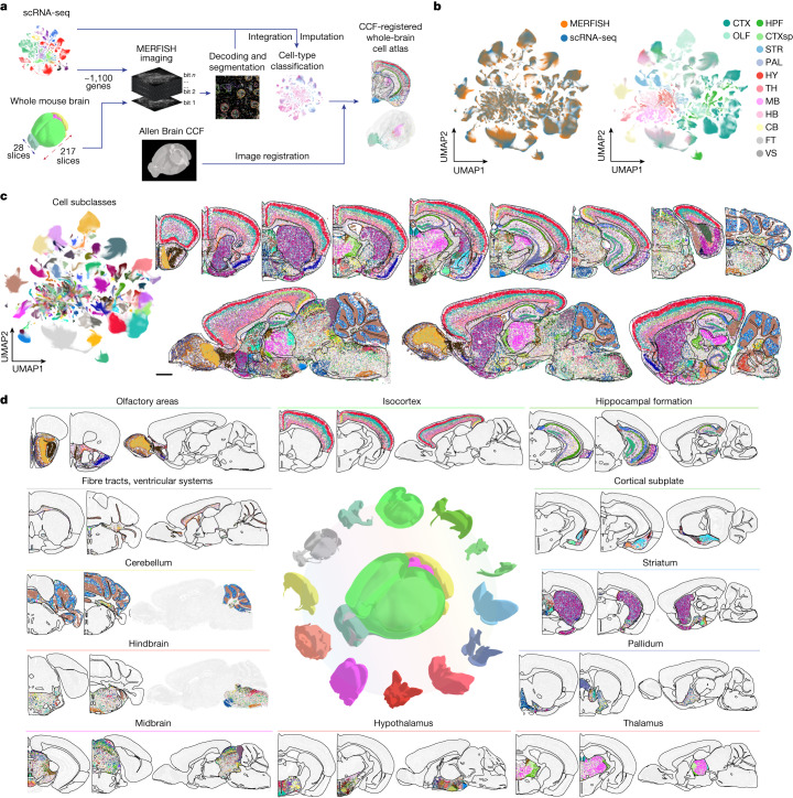
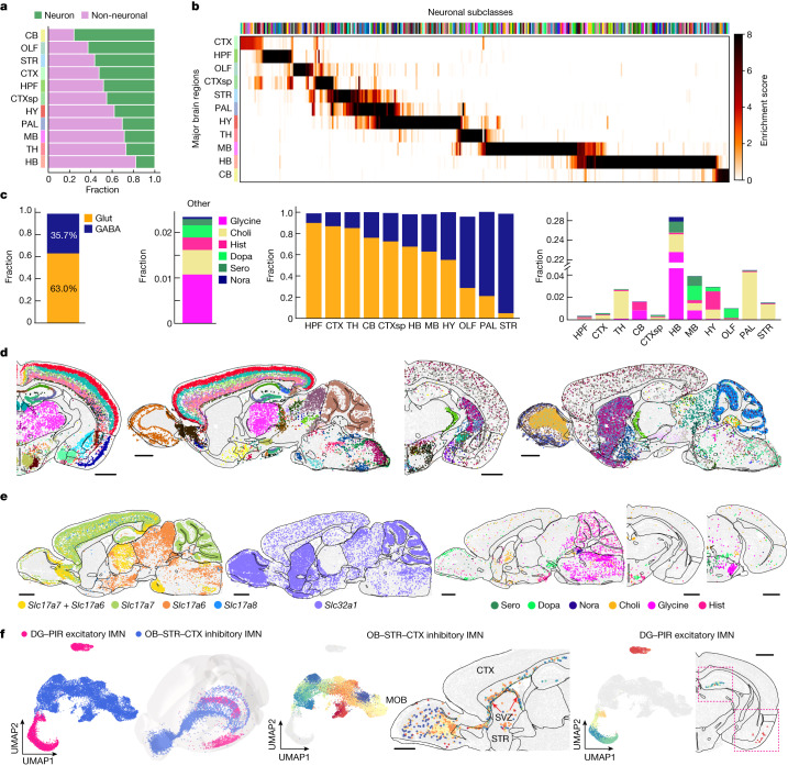
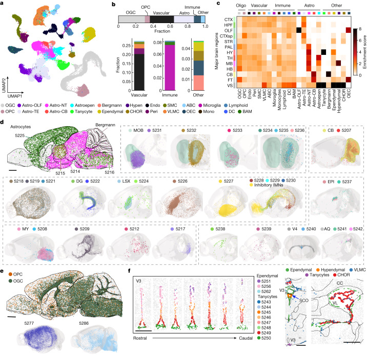
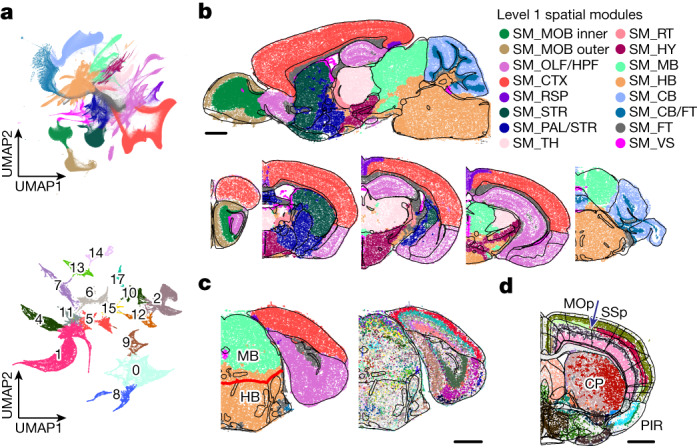
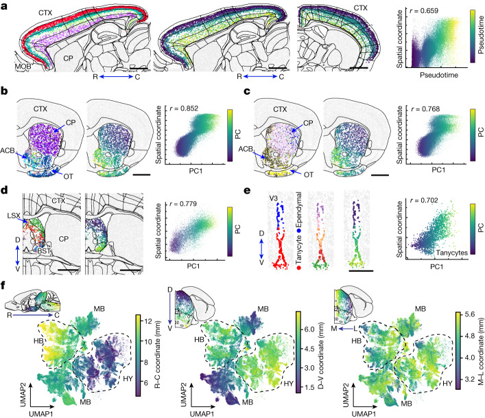
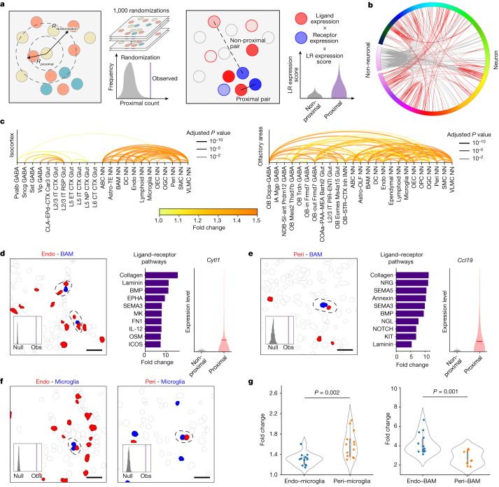
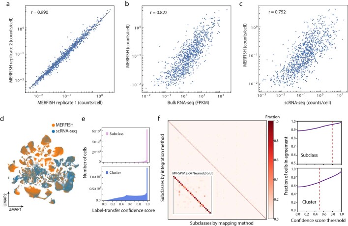
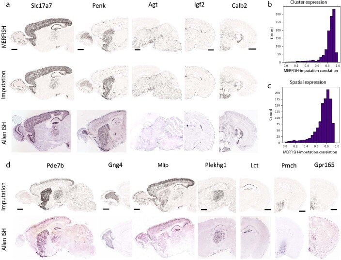
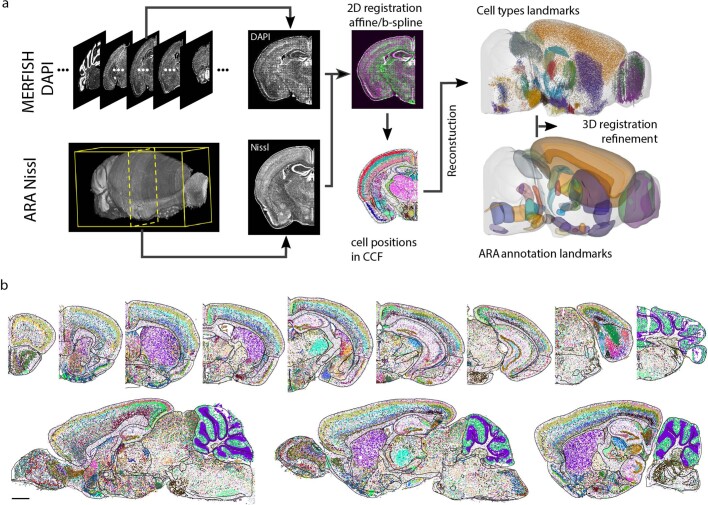
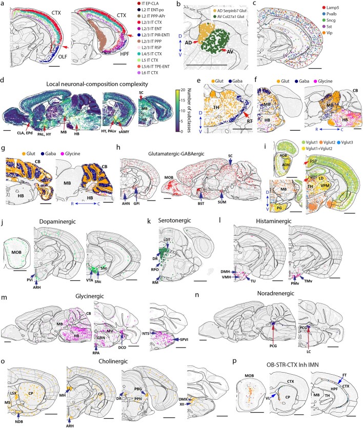
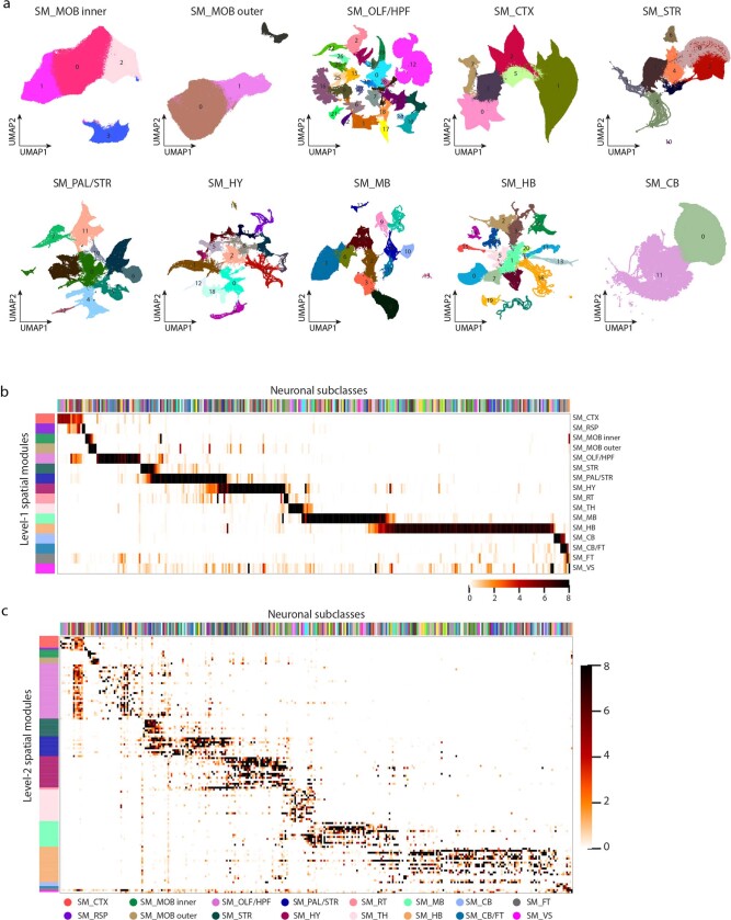
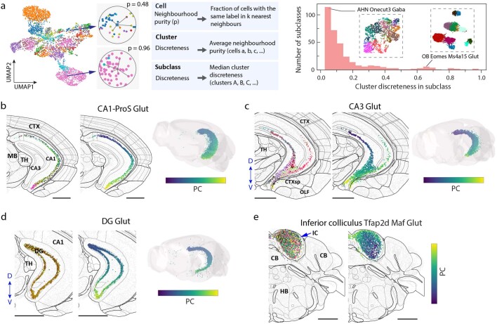
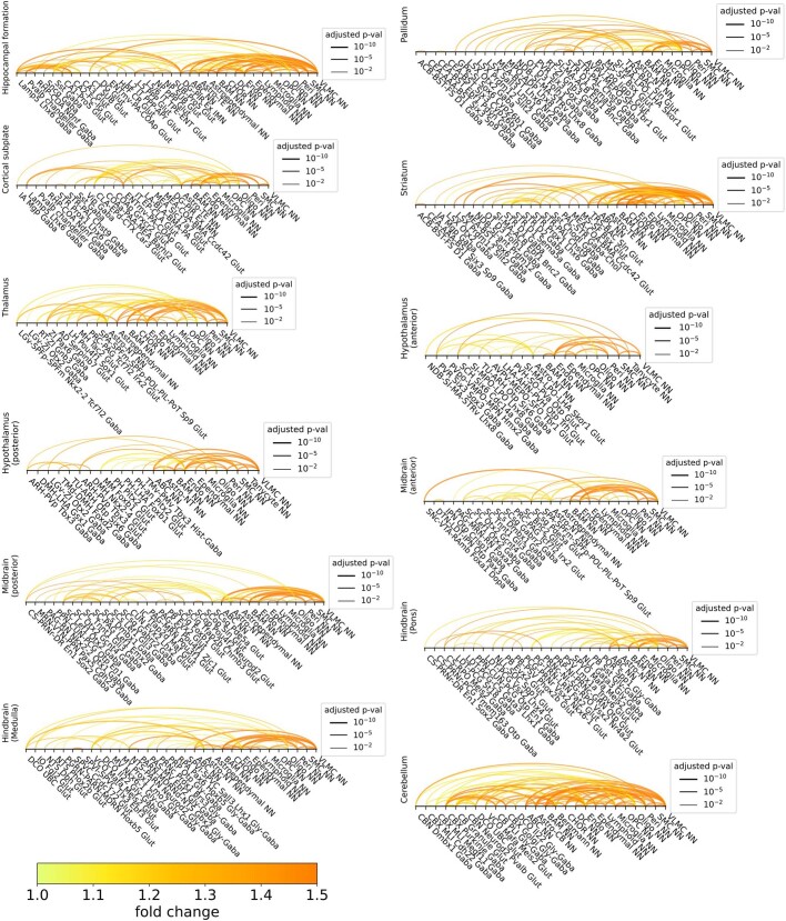
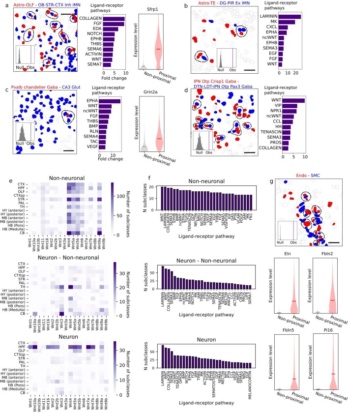
In mammalian brains, millions to billions of cells form complex interaction networks to enable a wide range of functions. The enormous diversity and intricate organization of cells have impeded our understanding of the molecular and cellular basis of brain function. Recent advances in spatially resolved single-cell transcriptomics have enabled systematic mapping of the spatial organization of molecularly defined cell types in complex tissues1-3, including several brain regions (for example, refs. 1-11). However, a comprehensive cell atlas of the whole brain is still missing. Here we imaged a panel of more than 1,100 genes in approximately 10 million cells across the entire adult mouse brains using multiplexed error-robust fluorescence in situ hybridization12 and performed spatially resolved, single-cell expression profiling at the whole-transcriptome scale by integrating multiplexed error-robust fluorescence in situ hybridization and single-cell RNA sequencing data. Using this approach, we generated a comprehensive cell atlas of more than 5,000 transcriptionally distinct cell clusters, belonging to more than 300 major cell types, in the whole mouse brain with high molecular and spatial resolution. Registration of this atlas to the mouse brain common coordinate framework allowed systematic quantifications of the cell-type composition and organization in individual brain regions. We further identified spatial modules characterized by distinct cell-type compositions and spatial gradients featuring gradual changes of cells. Finally, this high-resolution spatial map of cells, each with a transcriptome-wide expression profile, allowed us to infer cell-type-specific interactions between hundreds of cell-type pairs and predict molecular (ligand-receptor) basis and functional implications of these cell-cell interactions. These results provide rich insights into the molecular and cellular architecture of the brain and a foundation for functional investigations of neural circuits and their dysfunction in health and disease.


Conflict of interest statement

X.Z. is a co-founder and consultant of Vizgen. H.Z. is on the scientific advisory board of MapLight Therapeutics, Inc.

Figures

Fig. 1
Fig. 1. A molecularly defined and spatially resolved cell atlas of the whole mouse brain.
a, Workflow to construct a whole mouse brain cell atlas. A panel of genes were chosen for MERFISH imaging based on the clustering results from scRNA-seq data. MERFISH images were decoded and segmented, and the resulting single-cell gene expression profiles were integrated with scRNA-seq data to classify MERFISH cells and impute transcriptome-wide expression profiles. Finally, MERFISH images were registered to the Allen CCFv3 (ref. ). b, Uniform manifold approximation and projection (UMAP) of the integrated scRNA-seq and MERFISH data with cells coloured by experimental modalities (left) or by major brain regions in which the registered cells reside (right). The number of cells in the MERFISH or scRNA-seq dataset in each subclass was downsampled to the corresponding number in the other dataset for visualization purpose. The UMAP with all MERFISH and scRNA-seq cells displayed is shown in Extended Data Fig. 1d. CB, cerebellum; CTX, isocortex; CTXsp, cortical subplate; FT, fibre tract; HB, hindbrain; HPF, hippocampal formation; HY, hypothalamus; MB, midbrain; OLF, olfactory area; PAL, pallidum; STR, striatum; TH, thalamus; VS, ventricular system. c, UMAP of the integrated MERFISH and scRNA-seq data (left). Spatial maps of the cell types in example coronal and sagittal sections are also shown (right). Cells are coloured by their subclass identities. The black lines in the brain spatial maps here and in subsequent figures mark the major brain region boundaries defined in the CCF. Scale bar, 1 mm. In this and subsequent figures, all cells are shown in the experimental coordinates and the boundaries of brain regions were transformed to the experimental coordinates based on our CCF registration results (Methods). d, Spatial maps of example coronal and sagittal sections in the 11 major brain regions as well as in fibre tracts and ventricular systems. Cells are coloured by their subclass identities as in c. The underlying contour lines marking brain region boundaries in ac and d and the 3D brain contours in a and d were generated using coordinates from the Allen Mouse Brain CCFv3 (ref. ).
Fig. 2
Fig. 2. Cell-type compositions and spatial distributions of neurons.
a, Fractions of neurons and non-neuronal cells in the 11 major brain regions. b, Heatmap showing the enrichment score of each neuronal subclass in the 11 major brain regions. The enrichment score is defined as the fold change of the average cell density of a subclass within a brain region compared with the average density across the whole brain. c, Bar plots showing the fractions of neurons using different neurotransmitters across the whole brain (left two panels) and in individual brain regions (right two panels). Choli, cholinergic neuron; dopa, dopaminergic neuron; GABA, GABAergic neuron; glut, glutamatergic neuron; glycine, glycinergic neuron; hist, histaminergic neuron; nora, noradrenergic neuron; sero, serotonergic neuron. d, Spatial maps of the glutamatergic (left) and GABAergic (right) neuronal subclasses in example coronal and sagittal sections, with cells coloured by their subclass identities. e, Spatial maps of glutamatergic neurons expressing Slc17a7, Slc17a6, Slc17a7 + Slc17a6 and Slc17a8 (left), GABAergic neurons (middle) and neurons expressing various modulatory neurotransmitters (right). f, UMAP and spatial distribution of the immature neurons (IMNs) shown in the 3D CCF space, with cells coloured by subclass identities (left). UMAP and spatial distribution of the inhibitory IMNs shown in a sagittal section, with cells coloured by cluster identities (middle). Excitatory IMNs are shown in grey in the UMAP. UMAP and spatial distribution of the excitatory IMNs shown in a coronal section, with cells coloured by cluster identities (right). Inhibitory IMNs are shown in grey in the UMAP. Scale bars, 1 mm (df). DG, dentate gyrus; MOB, main olfactory bulb; PIR, piriform area; SVZ, subventricular zone. The red boxes mark the two locations of the excitatory IMNs in DG and PIR, respectively. The underlying contour lines marking brain region boundaries in df and the 3D brain contours in f were generated using coordinates from the Allen Mouse Brain CCFv3 (ref. ). Source Data
Fig. 3
Fig. 3. Cell-type compositions and spatial distributions of non-neuronal cells.
a, UMAP of non-neuronal cells coloured by subclass identities as shown in the legend. ABC, arachnoid barrier cell; astro, astrocyte; CHOR, choroid plexus epithelial cell; DC, dendritic cell; endo, endothelial cell; hypen, hypendymal cell; mono, monocytes; NT, non-telencephalic; OEC, olfactory ensheathing cell; OGC, oligodendrocyte; peri, pericytes; TE, telencephalic. Astro-OLF, Astro-TE, Astro-NT and Astro-CB are the subclasses of astrocytes located in the olfactory areas, telencephalic regions, non-telencephalic regions and cerebellum, respectively. b, Bar plots showing the fractions of major non-neuronal cell types in the whole brain (top). Fractions of different vascular cell types, immune cell types and non-neuronal cell types in the ‘other’ category with cell subclasses coloured as shown in the legend. c, Heatmap showing the enrichment scores of all non-neuronal subclasses in 11 major brain regions, as well as in fibre tracts and ventricular systems. The enrichment score is defined as in Fig. 2b. d, Spatial distributions of the 31 astrocyte clusters, which contained more than 50 cells (out of the 36 astrocyte clusters in total) and Bergmann cells, shown in a sagittal section (top left) and in the 3D CCF space (other panels), with cells coloured by cluster identities and cluster numerical indices. AQ, cerebral aqueduct; EPI, epithalamus; LSX, lateral septal complex; MY, medulla; V4, fourth ventricle. e, Spatial distributions of the OGCs and OPCs shown in a sagittal section with cells coloured by subclass identities (top). Two clusters are shown in the 3D CCF space (bottom). f, Spatial maps of three ependymal and eight tanycyte clusters in the third ventricle (V3) in seven coronal sections, 100 μm apart from each other along the rostral–caudal direction (left). Spatial maps of CHORs, ependymal cells, hypendymal cells and VLMCs in the third ventricle and lateral ventricle (VL) (right). Scale bars, 1 mm (d,e) and 0.5 mm (f). CC, corpus callosum; SCO, subcommissural organ. The underlying contour lines marking brain region boundaries in df and the 3D brain contours in d and e were generated using coordinates from the Allen Mouse Brain CCFv3 (ref. ). Source Data
Fig. 4
Fig. 4. Spatial modules: molecularly defined brain regions.
a, UMAP visualization of spatial modules. For any given cell, a local cell-type composition vector is calculated and used to cluster cells to determine the spatial modules (Methods). Level 1 spatial modules are determined with the cell-type composition determined at the subclass level; level 2 spatial modules are then determined for each level 1 spatial module with cell-type composition determined at both the subclass and the cluster levels and with only neurons considered. UMAP of cells in local cell-type composition space with cells coloured by their level 1 spatial module identities (top). UMAP of cells in one of the level 1 spatial modules (SM_TH, located at the thalamus) with cells coloured by their level 2 spatial module identities (bottom). b, Spatial maps of cells, coloured by their level 1 spatial module identities, shown in example sagittal and coronal sections. RSP, retrosplenial area; RT, reticular nucleus of the thalamus. c, Spatial maps of cells in one coronal section coloured by level 1 spatial module identities (left) and by cell subclass identities (right). The black lines mark the major brain region boundaries defined in the Allen CCF, and the CCF boundary between the midbrain and hindbrain is highlighted in red. d, Spatial map of cells coloured by level 2 spatial module identities in one coronal section. The black lines mark major brain region boundaries, and the thin grey lines mark the subregion boundaries defined in the CCF. The boundary between the primary motor cortex (MOp) and the primary somatosensory cortex (SSp) is indicated by the blue arrow. Scale bars, 1 mm (bd). CP, caudoputamen. The underlying contour lines marking brain region boundaries in bd were generated using coordinates from the Allen Mouse Brain CCFv3 (ref. ).
Fig. 5
Fig. 5. Spatial gradients of molecularly defined cell types.
a, Spatial gradient of IT neurons in the isocortex. From left to right: spatial map of IT neurons coloured by subclass identities in a sagittal section; spatial maps of IT neurons coloured by pseudotime in the same sagittal section and an additional coronal section; and a correlation plot of pseudotime versus cortical depth for individual IT neurons, coloured by pseudotime values. The Pearson correlation coefficient r is shown. C, caudal; R, rostral. b, Spatial gradient of the D1 medium spiny neurons (STR D1) in the striatum. From left to right: a spatial map of STR D1 neurons coloured by subclass identities in a coronal section; a spatial map of STR D1 neurons coloured by the first principal component (PC1) in the same coronal section; and a correlation plot of PC1 value versus spatial coordinate for individual STR D1 neurons, coloured by PC1 values. ACB, nucleus accumbens; OT, olfactory tubercle. ce, Same as b but for spatial gradients of STR D2 neurons in the striatum (c), GABAergic neurons in the LSX (d) and tanycytes in the third ventricle (V3) (e). BST, bed nuclei of the stria terminalis; D, dorsal; V, ventral. f, Large-scale gradient of neurons across the hypothalamus, midbrain and hindbrain. The UMAPs were generated based on the gene expression profiles of neurons, and individual cells are coloured by their spatial coordinates along the rostral–caudal (left), dorsal–ventral (middle) and medial (M)–lateral (L) (right) axes. The insets show example brain slices with cells in the regions of interest coloured by the relevant spatial coordinates. Scale bars, 1 mm (ad) and 0.5 mm (e). The underlying contour lines marking brain region boundaries in ad and f were generated using coordinates from the Allen Mouse Brain CCFv3 (ref. ). Source Data
Fig. 6
Fig. 6. Cell–cell interactions and communications.
a, Schematics of cell–cell interaction analysis (left) and ligand–receptor (LR) analysis (right). Rproximal denotes the proximity distance threshold; two cells are considered in contact or proximity if the distance between their centroid positions is within this distance threshold. Rrandomization denotes the randomization radius; we shifted the spatial location of each cell to a random position within R from its original location togenerate the null distribution. b, Cell–cell interactions across the whole brain. Each line corresponds to a predicted interacting cell-type pair. The grey lines indicate interactions between non-neuronal cells and neurons or among non-neuronal cells; the red lines indicate neuron–neuron interactions. c, Cell–cell interactions in two brain regions. Each line corresponds to an interacting cell-type pair, with the colour indicating fold change in proximity frequency compared with random chance and thickness indicating P values corrected by the Benjamini–Hochberg procedure. CLA, claustrum; CT, cortical-thalamic; EPd, endopiriform nucleus, dorsal part; ET, extratelencephalic; IT, intratelencephalic; L2/3, layer 2/3; NN, non-neuronal; NP, near-projecting. d, Interactions between endothelial cells and BAMs. Example image of cells, with cells of the indicated cell types shown in red and blue and all other cells shown in grey (left). Proximal cell pairs are circled by a dashed line. Observed counts (Obs) of the proximal cell pairs and the null distributions (null) from randomization control are shown in the inset. Top 10 ligand–receptor pathways upregulated in proximal cell pairs as compared to non-proximal cell pairs (middle). When multiple ligand–receptor pairs in a pathway are upregulated, the plotted fold-change value represents that of the pair with the highest upregulation fold change. Expression distributions of the indicated gene in endothelial cells proximal (red) or non-proximal (grey) to BAMs (right). Scale bar, 30 μm. Horizontal lines in the violin plots indicate median. e, Same as d, but for interactions between pericytes and BAMs. f, Interactions between endothelial cells and microglia (left) and between pericytes and microglia (right). g, Fold changes of observed proximal cell-pair number relative to the null-distribution mean across different brain regions. Each data point represents a brain region where significant interactions were observed (P values were calculated by two-sided Welch’s t-test; the centre points indicate the median, the boxes denote the interquartile range and the whiskers indicate 1.5 times the interquartile range). Comparison between endothelial–microglia and pericyte–microglia interactions (left), and comparison between endothelial–BAM and pericyte–BAM interactions (right). Source Data
Extended Data Fig. 1
Extended Data Fig. 1. Correlation and integration of MERFISH data and RNA-seq data.
a, Correlation plot of the average copy number per cell of individual genes measured by MERFISH from two replicate animals. The black solid line indicates equality. The Pearson correlation coefficient is r = 0.990. b, Correlation plot of the average copy number per cell of individual genes determined by MERFISH versus the expression levels determined by bulk RNA-seq of whole mouse brain. The Pearson correlation coefficient is r = 0.822. c, Correlation plot of the average copy number per cell of individual genes determined by MERFISH versus those determined by scRNA-seq of whole mouse brain. The Pearson correlation coefficient is r = 0.752. d, UMAP of the integrated MERFISH and scRNA-seq data with all MERFISH and scRNA-seq cells displayed. Cells are coloured by experimental modalities. e, Distributions of confidence scores of subclass label transfer (top) and cluster label transfer (bottom) for individual MERFISH cells. f, Left: Correspondence between the subclass classification of MERFISH cells determined by integration of MERFISH and scRNA-seq data (Integration method) and by identifying the scRNA-seq cluster with most similar transcriptional profile to the MERFISH cells (Mapping method). Confusion matrix shows the fraction of cells from any given subclass determined by the Integration method that was assigned to individual subclasses determined by the mapping method. Insets: Correspondence plots between the cluster classification of MERFISH cells determined by the two methods for an example subclass: MV-SPIV Zic4 Neurod2 Glut. Right: Fraction of cells showing classification agreement between the two methods as a function of the confidence score threshold at subclass level (top) and cluster level (bottom) used in the Integration method. Red dashed lines indicate the confidence score threshold used in this work. Source Data
Extended Data Fig. 2
Extended Data Fig. 2. Comparison of gene-expression results imputed from MERFISH and scRNA-seq data integration with the MERFISH measurement results and Allen in situ hybridization data.
a, Examples of spatial gene-expression patterns from MERFISH measurement (top row), imputation results (middle row), and in situ hybridization data from the Allen brain atlas (bottom row). b,c, The distributions of Pearson correlation coefficients between MERFISH measurement results and imputation results. b, For each gene, a correlation coefficient was calculated for mean expression levels in individual cell clusters between MERFISH measurement results and imputation results. c, For each gene, a correlation coefficient was calculated for mean expression levels of individual imaging fields of view (200 µm × 200 µm) between MERFISH measurement results and imputation results. Correlation-coefficient distributions across all genes in the MERFISH panel are shown. d, Examples of spatial gene expression patterns from imputation results (top row) and in situ hybridization data from the Allen brain atlas (bottom row). The genes shown in (d) were not measured by MERFISH. Scale bars in a,d: 1 mm. The Allen Brain Atlas in situ hybridization data in panels a and d  are taken from https://mouse.brain-map.org/. Source Data
Extended Data Fig. 3
Extended Data Fig. 3. CCF registration of MERFISH images.
a, Workflow of CCF registration of the MERFISH images. MERFISH images were registered to the Allen Mouse Brain CCFv3 using a two-step procedure. First, DAPI images taken during MERFISH imaging were aligned to the Nissl template images in the Allen Reference Atlas (ARA, adapted from https://mouse.brain-map.org/static/atlas), which allowed an initial, coarse alignment of the MERFISH images to the Allen CCF. Second, cell-type with known locations in the CCF were selected as landmarks (e.g., layer-specific cortical neurons, neurons in the dente gyrus, etc.) and used to refine the CCF alignment (see Methods for details). The 3D brain images were generated using Brainrender. b, Spatial maps of cells in the same coronal and sagittal sections as shown in Fig. 1c, but with cells coloured by their cluster identities. The underlying contour lines marking the brain region boundaries were generated using coordinates from the Allen Mouse Brain CCFv3 (ref. ). Scale bar: 1 mm.
Extended Data Fig. 4
Extended Data Fig. 4. Spatial distributions of different neuronal cell types and neurotransmitter usage.
a, Spatial distributions of different IT subclasses showing the separation between IT neurons in the isocortex (CTX) and those in the olfactory areas (OLF, left) and in the hippocampal formation (HPF, right). Red arrows mark the boundaries between CTX and OLF and between CTX and HPF defined in the CCF. Cells are coloured by subclass identities. b, Spatial distributions of the two subclasses, AD Serpinb7 Glut and AV Col27a1 Glut, in the anterodorsal (AD) and anteroventral (AV) nucleus of the thalamus, respectively. c, Spatial distributions of five inhibitory neuronal subclasses, marked by Lamp5, Pvalb, Sst, Vip, and Sncg, across CTX, HPF, OLF and cortical subplate (CTXsp). d, Spatial heatmap of local neuronal-composition complexity. The local neuronal-composition complexity of any given cell is defined as the number of different neuronal cell types (at the subclass level) present in the 50 nearest-neighbour neurons surrounding that cell. PAL, Pallidum; PALv, Pallidum, ventral region; sAMY, Striatum-like amygdalar nuclei; SC, Superior colliculus. e, Spatial distributions of glutamatergic and GABAergic neurons in the thalamus, showing GABAergic neurons in the reticular nucleus (RT) and glutamatergic neurons in the rest of the thalamus. f, Spatial distributions of glutamatergic and GABAergic neurons, including the glycinergic neurons, in the midbrain and hindbrain. g, Spatial distributions of glutamatergic and GABAergic neurons, including the glycinergic neurons, in the cerebellum. h, Spatial distributions of neurons co-expressing Vglut (Slc17a6, Slc17a7 or Slc17a8) and Vgat (Slc31a1). AHN, Anterior hypothalamic nucleus; GPi, Globus pallidus, internal segment; SUM, Supramammillary nucleus. i, Spatial distributions of neurons expressing Vglut1 (Slc17a7, green) and Vglut2 (Slc17a6, orange). Neurons that co-express Vglut1 and Vglut2 are shown in yellow. AOB, Accessory olfactory bulb; AON, Anterior olfactory nucleus; MH, Medial habenula; LD, Lateral dorsal nucleus of thalamus; VPM, Ventral posteromedial nucleus of the thalamus; PG: Pontine gray. jo, Spatial distributions of dopaminergic (j), serotonergic (k), histaminergic (l), glycinergic (m), noradrenergic (n) and cholinergic (o) neurons. PVi, Periventricular hypothalamic nucleus, intermediate part; ARH, Arcuate hypothalamic nucleus; VTA, Ventral tegmental area; SNr, Substantia nigra, reticular part; SNc, Substantia nigra, compact part; LDT, Laterodorsal tegmental nucleus; DMH, Dorsomedial nucleus of the hypothalamus; VMH, Ventromedial hypothalamic nucleus; TU, Tuberomammillary nucleus; PMv, Ventral premammillary nucleus; TMv, Tuberomammillary nucleus, ventral part; MV, Medial vestibular nucleus; GRN, Gigantocellular reticular nucleus; RPA, Nucleus raphe pallidus; DCO, Dorsal cochlear nucleus; NTS, Nucleus of the solitary tract; SPVI, Spinal nucleus of the trigeminal, interpolar part; PCG, Pontine central gray; LC, Locus ceruleus; MS, Medial septal nucleus; NDB, Diagonal band nucleus; PBG, Parabigeminal nucleus; PPN, Pedunculopontine nucleus; DMX, Dorsal motor nucleus of the vagus nerve; XII, Hypoglossal nucleu. p, Spatial distribution of the inhibitory immature neurons (IMNs) coloured by cluster identities as in Fig. 2f middle panel. Scale bars in ap: 1 mm. The underlying contour lines marking brain region boundaries in ap were generated using coordinates from the Allen Mouse Brain CCFv3 (ref. ).
Extended Data Fig. 5
Extended Data Fig. 5. Spatial distributions of neuropeptide usage.
Spatial distributions of neurons expressing various neuropeptide genes shown in multiple example coronal slices. Scale bar: 1 mm. The underlying contour lines marking brain region boundaries in the images were generated using coordinates from the Allen Mouse Brain CCFv3 (ref. ).
Extended Data Fig. 6
Extended Data Fig. 6. Spatial distributions of additional non-neuronal cell types.
a, Left: Spatial distributions of VLMCs shown in an example coronal section. Right: Spatial distributions shown in the 3D CCF space for VLMC cluster 5301 (top), which is enriched in the grey matter, and cluster 5302 (bottom), which is located in the choroid plexus in the lateral and fourth ventricles. b, Spatial distributions of arachnoid barrier cells (ABCs) shown in an example coronal section. c, Spatial distributions of endothelial cells (left), pericytes (middle) and smooth muscle cells (SMCs, right), each shown in an example coronal section. d, Spatial distributions of immune cells shown in an example coronal section including microglia (left) and in the same section but without showing microglia (right). e, Spatial distributions of olfactory ensheathing cells (OEC) shown in an example coronal section. Cells are coloured by cluster identities in all panels. Scale bars in ae: 1 mm. The underlying contour lines marking brain region boundaries in ae and the 3D brain contours in a were generated using coordinates from the Allen Mouse Brain CCFv3 (ref. ).
Extended Data Fig. 7
Extended Data Fig. 7. Spatial-module delineation.
a, UMAP of cells in the other level-1 spatial module, as in Fig. 4abottom, with cells coloured by their level-2 spatial module identity. b,c, Heatmaps showing the enrichment scores of all neuronal subclasses in the 16 level-1 spatial modules (b) and in the 130 level-2 spatial modules (c). The enrichment score is defined as the fold change of the fraction of cells belong to a subclass in each individual spatial module compared to the same fraction across all spatial modules. The coloured bars at the top and on the left indicate the neuronal subclasses and spatial modules, respectively. Source Data
Extended Data Fig. 8
Extended Data Fig. 8. Quantification of cluster discreteness of cell subclasses and additional examples of spatial gradients of molecularly defined cell types.
a, Left: To quantify the cluster discreteness in a subclass, a neighbourhood purity quantity for each cell in a cluster is determined as the fraction of the cells in its neighbourhood (in the gene-expression space) that belong to this cluster. The mean neighbourhood purity quantity across all cells in a cluster is defined as the discreteness of the cluster, which gives a measure of how well separated this cluster is from the other clusters in the gene-expression space. The median discreteness of clusters is then determined for each subclass. Right: Distribution of the median cluster discreteness of individual subclasses across all subclasses. The UMAPs of an example subclass with high cluster discreteness (OB Eomes Ms4a15 Glut) and an example subclass with low cluster discreteness (AHN Onecut3 Gaba) are shown. bd, Spatial gradients of CA1-Pros Glut neurons (b), CA3 Glut neurons (c) and DG Glut neurons (d) in the hippocampal formation. From left to right: Spatial map of cells coloured by cluster identities in a coronal section; Spatial map of cells coloured by the first principal component (PC1) in the same section; Spatial distribution of cells colored by PC1 shown in the 3D CCF space. e, Spatial gradient of the Tfap2d Maf Glut neurons in the inferior colliculus (IC) of the midbrain. Cells are shown in one coronal section and are coloured by cluster identities (left) and PC1 (right). Scale bars in be: 1 mm. The underlying contour lines marking brain region boundaries in be and the 3D brain contours in bd were generated using coordinates from the Allen Mouse Brain CCFv3 (ref. ). Source Data
Extended Data Fig. 9
Extended Data Fig. 9. Predicted cell-cell interactions or communications in individual brain regions.
Same as in Fig. 6c, but for the hippocampal formation, cortical subplate, striatum, pallidum, thalamus, hypothalamus (anterior and posterior parts), midbrain (anterior and posterior parts), hindbrain (pons and medulla sub-regions), and cerebellum.
Extended Data Fig. 10
Extended Data Fig. 10. Additional examples and characterizations of predicted cell-cell interactions or communications.
a, Interactions between olfactory astrocytes (Astro-OLF) and inhibitory immature neurons (MOB-STR-CTX inh IMN). Left: Example image of cells in a small area, with cells belonging to the indicated cell types shown in red and blue and all other cells shown in grey, as described in Fig. 6d. Middle: Top 10 upregulated ligand-receptor pathways, as described in Fig. 6d. Right: Expression distributions of the indicated gene in Astro-OLF proximal (red) or non-proximal (grey) to MOB-STR-CTX inh IMN, as described in Fig. 6d. bd, Same as a, but for interactions between astrocytes (Astro-TE) and excitatory immature neurons (DG-PIR Ex IMN) (b), between Pvalb chandelier Gaba neurons and CA3 Glut neurons (c), and between IPN Otp Crisp1 Gaba neurons and DTN-LDT-IPN Otp Pax3 Gaba neurons (d). In (b) and (d), violin plots of example genes upregulated in proximal cell pairs as compared to non-proximal cell pairs are not shown. e, Total numbers of unique cell types (subclasses) observed in the interacting cell-type pairs that showed upregulation of the ligand-receptor pairs involving the indicated Wnt ligands in each of the major brain regions. Top: For interactions among non-neuronal cells; Middle: For interactions between neurons and non-neuronal cells; Bottom: For interactions among neurons. f, The total number of unique cell-types (subclasses) involved in the predicted interacting cell-type pairs that showed upregulation of ligand-receptor pairs in the indicated pathway across the whole brain. For each category of cell-cell interactions (interactions among non-neuronal cells (top), interactions between neurons and non-neuronal cells (middle), and interactions among neurons (Bottom)), the top 30 ligand-receptor pathways with the highest number of cell types involved are shown. g, Interactions between endothelial cells and SMC cells. Top: Example image of cells in a small area, as described in Fig. 6d. Bottom: Expression distributions of the indicated genes in endothelial cells when they are proximal or non-proximal to SMC. Scale bars in a,b,e: 30 μm. Source Data

Update of

Similar articles

Cited by

References

    1. Larsson L, Frisen J, Lundeberg J. Spatially resolved transcriptomics adds a new dimension to genomics. Nat. Methods. 2021;18:15–18. doi: 10.1038/s41592-020-01038-7. - DOI - PubMed
    1. Zhuang X. Spatially resolved single-cell genomics and transcriptomics by imaging. Nat. Methods. 2021;18:18–22. doi: 10.1038/s41592-020-01037-8. - DOI - PMC - PubMed
    1. Close JL, Long BR, Zeng H. Spatially resolved transcriptomics in neuroscience. Nat. Methods. 2021;18:23–25. doi: 10.1038/s41592-020-01040-z. - DOI - PubMed
    1. Moffitt JR, et al. Molecular, spatial, and functional single-cell profiling of the hypothalamic preoptic region. Science. 2018;362:eaau5324. doi: 10.1126/science.aau5324. - DOI - PMC - PubMed
    1. Wang X, et al. Three-dimensional intact-tissue sequencing of single-cell transcriptional states. Science. 2018;361:eaat5691. doi: 10.1126/science.aat5691. - DOI - PMC - PubMed

LinkOut - more resources