. 2023 Dec;624(7991):403-414.
doi: 10.1038/s41586-023-06817-8. Epub 2023 Dec 13.

A transcriptomic taxonomy of mouse brain-wide spinal projecting neurons

Affiliations

A transcriptomic taxonomy of mouse brain-wide spinal projecting neurons

Carla C Winter et al. Nature. 2023 Dec.

Abstract

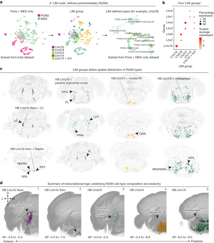
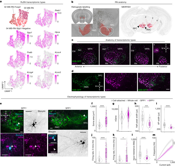
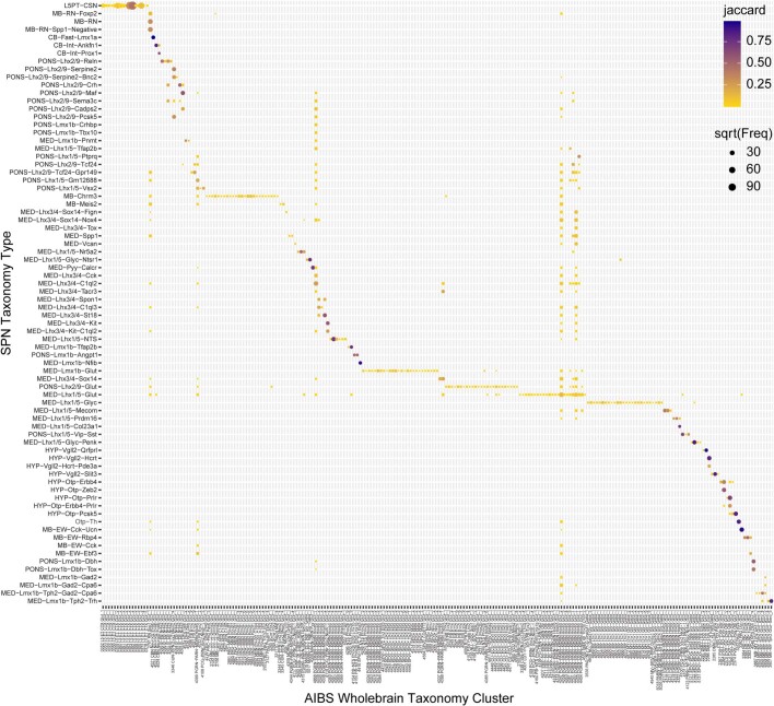
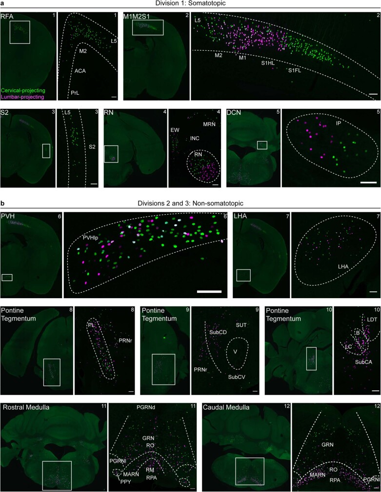
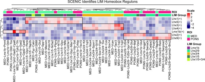
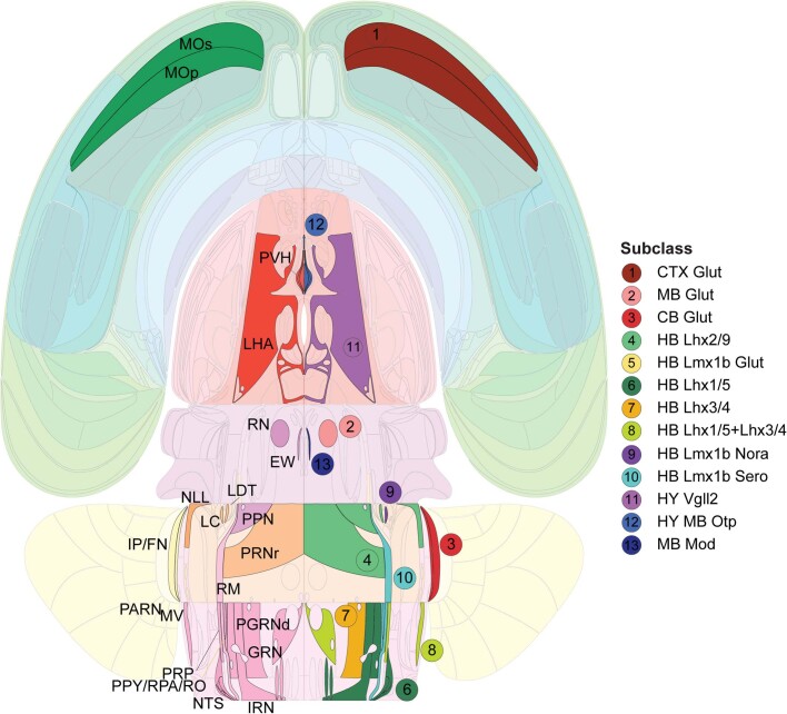
The brain controls nearly all bodily functions via spinal projecting neurons (SPNs) that carry command signals from the brain to the spinal cord. However, a comprehensive molecular characterization of brain-wide SPNs is still lacking. Here we transcriptionally profiled a total of 65,002 SPNs, identified 76 region-specific SPN types, and mapped these types into a companion atlas of the whole mouse brain1. This taxonomy reveals a three-component organization of SPNs: (1) molecularly homogeneous excitatory SPNs from the cortex, red nucleus and cerebellum with somatotopic spinal terminations suitable for point-to-point communication; (2) heterogeneous populations in the reticular formation with broad spinal termination patterns, suitable for relaying commands related to the activities of the entire spinal cord; and (3) modulatory neurons expressing slow-acting neurotransmitters and/or neuropeptides in the hypothalamus, midbrain and reticular formation for 'gain setting' of brain-spinal signals. In addition, this atlas revealed a LIM homeobox transcription factor code that parcellates the reticulospinal neurons into five molecularly distinct and spatially segregated populations. Finally, we found transcriptional signatures of a subset of SPNs with large soma size and correlated these with fast-firing electrophysiological properties. Together, this study establishes a comprehensive taxonomy of brain-wide SPNs and provides insight into the functional organization of SPNs in mediating brain control of bodily functions.


Conflict of interest statement

Z.H. is an advisor of SpineX, Life Biosciences, and Myro Therapeutics. H.Z. is on the scientific advisory board of MapLight Therapeutics, Inc. The remaining authors declare no competing interests.

Figures

Fig. 1
Fig. 1. An anatomically informed transcriptomic atlas of brain-wide spinal projecting neurons.
a, SPNs were labelled via spinal cord injections of a retrograde AAV construct that localizes fluorescent protein expression to the nucleus for parallel anatomical and transcriptomic profiling. Test tubes were drawn using templates from Servier Medical Art (Creative Commons Attribution 3.0 Unported Licence https://creativecommons.org/licences/by/3.0/). The sagittal atlas outline was adapted from the Allen Mouse Brain Atlas (https://atlas.brain-map.org/); ©2017 Allen Institute for Brain Science. b, WB reconstructions of segmented and registered SPN nuclei imaged with STPT revealed that SPNs are present across the CTX (RFA, M1M2S1 and S2), HY, MB, CB, PONS and MED. c, Multilevel iterative clustering revealed 76 SPN transcriptomic ‘types’ organized into a taxonomy across 13 ‘subclasses’ and 3 ‘divisions’ (n = 61,484 10x; n = 3,518 SSv4). The colour blocks shading the taxonomy tree indicate division. The nodes at the end of the dendrogram indicate type, with type numbers and names on the far right. From left to right, the bar plots indicate subclass, fractions of nuclei profiled from brain region-enriching dissections and NT-type across each type. The heatmap shows expression of neurotransmitter marker genes. The bar plot below the division legend indicates percentage of total nuclei belonging to each division. df, Clustering of SPNs and visualization in UMAP space coloured by brain ROI-enriching dissections (d), division (e) and subclass (f). ROI, division, and subclass colours in c apply to d,e and f, respectively. Percentage labels in d and e indicate percentage of total nuclei belonging to each ROI-enriching dissection or division. NT-type, neurotransmitter type.
Fig. 2
Fig. 2. SPNs from cortical layer 5, red nucleus and cerebellum are transcriptionally and anatomically discrete.
a, UMAP of all SPNs, coloured by types within taxonomy division 1. b, Expression of select genes for neurotransmission machinery. ce, Expression of select marker genes (top) and representative MERFISH sections (bottom) of corticospinal neurons (c), rubrospinal neurons (d) and cerebellospinal neurons (e). Number labels depicted on the MERFISH panels correspond to SPN types in a and in the global dendrogram in Fig. 1c. f, Confocal microscopy images of retrogradely labelled cervical- (green) and lumbar- (magenta) projecting corticospinal neurons (1), rubrospinal neurons (2) and cerebellospinal neurons (3). Scale, 100 µm. Representative images shown here from n = 3 injected mice. Expression scale in b applies to all expression plots. FN, fastigial nucleus; IP, interposed nucleus; RN, red nucleus; S1FL, primary somatosensory cortex forelimb region; S1HL, primary somatosensory cortex hindlimb region.
Fig. 3
Fig. 3. Diverse neurotransmitter identities of SPNs.
a, UMAP of all SPNs, coloured by subclasses within taxonomy division 3. b, Subset UMAP (left) and MERFISH representation (right) of types within HY MB Otp subclass. Bottom right, expression of Th and additional monoaminergic markers. c, Subset UMAP (left) and MERFISH representation (right) of types within HY Vgll2 subclass. d, Subset UMAP (left) and MERFISH representation (middle) of types within the MB Mod subclass. Expression of select marker genes (right). e,f, Same as d but for types in HB Lmx1b Nora and Sero subclasses (e) and type MED-Lhx1/5-NTS (f). Expression scale in b applies to all expression plots. Types coloured and assigned number labels as in Fig. 1c.
Fig. 4
Fig. 4. LIM homeobox genes parcellate reticulospinal neurons into spatially and transcriptionally distinct subsets.
a, Nuclei from PONS- and MED-enriching dissections were subset and re-embedded (10x data, n = 22,100 nuclei). Left/middle, UMAP of nuclei from PONS- and MED-enriching dissections coloured by ROI and LIM groups, respectively. Right, each LIM group was subset and re-embedded to identify the final types depicted in Fig. 1c. Shown here is the re-embedding of the Lhx2/9 group. b, Dot plot showing expression of Lmx1bLhx2Lhx9Lhx3Lhx4Lhx1 and Lhx5 grouped by the five LIM groups. c, Representative MERFISH sections of ReSN types, each coloured by their respective LIM-defined subclass. d, Anatomical distributions of LIM-defined subclasses summarized using representative coronal reconstructions of Cre-dependent retrogradely labelled nuclei in transgenic lines corresponding to LIM-defined subclasses (from Extended Data Fig. 9). Panel 1: Dbh-Cre, TH-Cre and Phox2b-Cre, coloured as HB Lmx1b Nora subclass. Panel 2: ePet-Cre, coloured as HB Lmx1b Sero subclass. Panel 3: Lhx2-2A-CreER, coloured as HB Lhx2/9 subclass. Panel 4: Chx10-Cre, coloured as HB Lhx3/4 subclass. Panel 5: ChAT-Cre, GlyT2-Cre, and Gcg-iCre, coloured as HB Lhx1/5 subclass. AP, anterior–posterior position (relative to Bregma); B, Barrington’s nucleus; LC, locus coeruleus; LDT, laterodorsal tegmental nucleus; IRN, intermediate reticular nucleus; PARN, parvicellular reticular nucleus; PL, paralemniscal nucleus (Paxinos nomenclature); PPN, pedunculopontine nucleus; PPY, parapyramidal nucleus; PRNr, pontine reticular nucleus rostral part; RF, reticular formation; RM, nucleus raphe magnus; RO, nucleus raphe obscurus; RPA, nucleus raphe pallidus; SubCD/CV/CA, subcoeruleus nucleus dorsal/ventral/alpha parts (Paxinos).
Fig. 5
Fig. 5. Transcriptomic differences among SPNs terminating at different spinal targets.
a, The 10x data were generated by separately collecting cervical-projecting (GFP+) from dual- (GFP+/mScarlet+) and lumbar- (mScarlet+) projecting SPNs nuclei across the WB, and the SSv4 dataset used indexed plate-based sorting to separate cervical- (GFP+), lumbar- (mScarlet+) and dual- (GFP+/mScarlet+) projecting SPNs. b, UMAP visualization of all SPNs coloured by source (ROI, as in Fig. 1d) and target (spinal cord level). c, Proportion of cervical (green) versus dual or lumbar (pink) across SPN transcriptomic types. Bars above proportion plot indicate subclass and division. Types ordered as in Fig. 1c. d, Violin plot of the differentially expressed genes Epha4 and Efna5 across all SPNs, grouped by ROI (10x data, n = 61,484 nuclei). The centre line of the overlayed box and whisker plots depicts the median value (50th percentile) while the box contains the 25th to 75th percentiles; the whiskers correspond to the 5th and 95th percentiles. e, Proportion of cervical-, dual- and lumbar-projecting neurons in the SSv4 CSN and RuSN datasets. f, SSv4 UMAPs of CSNs (top) and RuSNs (bottom). g, Volcano plots of differentially expressed genes for cervical- (green) versus dual-/lumbar- (magenta) projecting CSNs (top) and RuSNs (bottom). Genes of interest are labelled. Differential expression analysis was performed with Seurat using the MAST test; significant genes were defined as those with a false discovery rate adjusted P value of less than 0.05. h, enrichR was used to determine enriched Gene Ontology terms of differentially expressed genes in g in CSNs (top) and RuSNs (bottom). enrichR uses adjusted P values computed using the Benjamini–Hochberg method for correction for multiple hypotheses testing.
Fig. 6
Fig. 6. Anatomy, morphology and electrophysiology of rubrospinal types.
a, UMAP of RuSNs (SSv4, n = 1,031 nuclei) coloured by type (top left) and expression of general RuSN marker gene (Rreb1, top right). Expression of differentially expressed genes for SPP1+ (Spp1, Pvalb, Kcng4; left, bottom three) and SPP1 (Hpca, Kcnc4, Kcnn3; right, bottom three) RuSNs. b, Left, coronal reconstruction of  RuSNs imaged with STPT. Right, MERFISH mapping depicting types 02–04 (same as Fig. 2). c, Representative IHC results for SPP1 on retrogradely labelled RuSNs. d, Expanded view of panel 2 in c. Scale, 100 µm. n = 3 brains stained to yield representative results. e, Confocal images of representative SPP1+ and SPP1− RuSNs in slices from cell-attached recordings. Biocytin was injected into recorded cells and labelled with fluorophore-conjugated streptavidin. Scale, 50 µm. f, Quantification of soma size from cell-attached and whole-cell recordings. g, Number of genes detected in RuSNs (SSv4, n = 1,031 nuclei). h, Half-peak width of spike waveforms from cell-attached recordings. im, Action potential width (i), spontaneous firing rate at 0 min (j) and 5 min (k), input resistance (l), and frequency–current injection (m) from whole-cell recordings. **** P < 0.0001, *** P < 0.001, ** P < 0.01, * P < 0.05, Mann–Whitney test (two-sided) (f,hl); generalized linear mixed effect model (two-sided) (m). In fl, the centre line of the box plot depicts the median value while the box contains the 25th–75th percentiles; whiskers correspond to the 5th and 95th percentiles. In m, the solid line shows mean firing frequency and shaded area shows s.e.m. Number of cells and statistical tests are summarized in Supplementary Table 13. 3N, cranial nerve 3; INC, interstitial nucleus of Cajal; MRN, MB reticular nucleus; RMC, magnocellular red nucleus; RPC, parvocellular red nucleus. Source Data
Extended Data Fig. 1
Extended Data Fig. 1. Spinal injection sites of adeno-associated viruses for nuclear labelling.
Recombinant AAVs were injected into multiple segments centring on the cervical and lumbar spinal cord of P42 C57BL/6J mice. Mice were euthanized 2 weeks later at P56. a-c, Representative horizontal (i.e., dorsal-ventral longitudinal) sections of spinal cords injected with AAV2/2-H2B into cervical levels 4-6 (C4-6) and lumbar levels 2-4 (L2-4). AAV2/2-H2B does not retrogradely label neurons and therefore labels cells only local to spinal injection sites. b and c are zoom-in of dashed boxed in a. d-f, Representative horizontal sections of spinal cords injected with AAV2/retro-H2B into C4-6 and L2-4. AAV2/retro-H2B, the viral vector used to retrogradely label spinal projecting neurons, has retrograde labeling capability and therefore the spinal injection sites depict both locally transduced cells and retrogradely labelled intraspinal projection neurons (i.e., propriospinal neurons). e and f are zoom-in of dashed boxed in d. g-h, Representative coronal sections of (g) cervical and (h) lumbar spinal injection sites labelled by AAV2/retro-H2B demonstrating labeling in ventral horn, dorsal horn, and intermediate zone of the spinal cord grey matter (marked by dashed outline). N = 3 spinal cords were labelled with AAV2/2-H2B and N = 3 spinal cords were labelled with AAV2/retro-H2B to yield representative images shown here. Scale a-f , 1000 µm; scale g-h , 200 µm.
Extended Data Fig. 2
Extended Data Fig. 2. Anatomical overview of spinal projecting neurons.
a, Coronal reconstructions (250 µm thickness) of segmented and registered SPN nuclei imaged with STPT. b, Bar plots represent percentages of SPNs profiled from each SPN-containing brain region in snRNA-seq (10x and SSv4; number of nuclei in each ROI-enriching dissection are as follows, M1M2S1 : 20612, RFA: 5876, S2: 3354, MED: 15264, PONS: 7913, MB: 6834, HY: 3696, CB: 1453) and histological datasets (slide-scanner imaging; N = 5 mice, mean and standard deviation for number of nuclei in each ROI are as follows, RFA: 5586.40 +/− 425.76, S2: 2188.80 +/− 101.84, M1M2S1 : 25925.60 +/− 857.80, HY: 2337.60 +/− 267.77, MB: 10394.40 +/− 654.72, CB: 1757.60 +/− 265.87, PONS: 12916.80 +/− 1124.68, MED: 19570.40 +/− 465.30). Legend for (a) and (b) is depicted in upper right corner (same as panel Fig. 1b). Source Data
Extended Data Fig. 3
Extended Data Fig. 3. High-throughput isolation of retrogradely labelled spinal projecting neurons for snRNA-seq.
a, Regions containing retrogradely labelled SPNs were dissected from P56 mice. A 1 mm coronal-oriented brain matrix was used to section brains from the olfactory bulb to Lambda, and a sagittal-oriented matrix was used to section the remaining subcortex. Test tubes were drawn using templates from Servier Medical Art (Creative Commons Attribution 3.0 Unported License https://creativecommons.org/licences/by/3.0/). Sagittal atlas outline adapted from Allen Institute for Brain Science (https://mouse.brain-map.org/static/atlas). b, Dissection scheme was based on STPT imaging, which shows the cleanest dissection planes to separate the major regions containing SPNs are coronal for forebrain (i) and sagittal for midbrain and hindbrain (same as panel Fig. 1b) (ii). Equal numbers of male and female mice were pooled per ROI to input sufficient nuclei for FANS (iii). Panel b is same as in Fig. 1b. c, Example dissecting microscope images showing the dissection planes based on the scheme in a and b. Estimated scale based on Paxinos adult mouse brain atlas, ~1000 µm. This scheme was used to dissect the N = 30 mice from which the snRNA-seq datasets were generated (donor information summarised in Supplementary Table 1). d, Following microdissection, nuclei were isolated from each ROI and SPNs enriched using FANS. Representative plots shown are from an M1M2S1 sample. e, Enrichment for GFP+ and/or mScarlet+ nuclei was confirmed post-FANS. Scale, 100 µm. Box plot depicts the proportion of sorted nuclei (labelled with DAPI) that had detectable GFP and/or mScarlet via widefield microscopy (N = 4 M1M2S1 samples). The centre line of the box plot depicts the median value (50th percentile) while the box contains the 25th to 75th percentiles; whiskers correspond to the 5th and 95th percentiles. Rep, replicate. Source Data
Extended Data Fig. 4
Extended Data Fig. 4. Identification of first- and second-order retrogradely labelled nuclei.
a, The proportion of labelled nuclei were quantified in the cortex, revealing 96.76% and 3.24% of nuclei were labelled within and outside of L5CTX, respectively (N = 5 mice, mean and standard deviation are as follows, L5CTX: 33700.80 + /- 929.89, Upper CTX: 882.40 + /-296.89, Lower CTX: 246.40 + /-147.61). b, Qualitative assessment shows lower fluorescence intensity of nuclei in non-L5CTX compared to L5CTX (Cervical: N = 17 lower CTX, 5082 M1M2S1, 42 upper CTX; Lumbar: N = 25 lower CTX, 2606 M1M2S1, 123 upper CTX across 1 retrogradely labelled sample). Arrows indicate faintly labelled nuclei. Scale, 200 µm. c, Box plot depicting fluorescence intensity of GFP- and mScarlet- labelled nuclei is significantly higher in L5CTX compared to upper (layers 1–4) and lower (layer 6) cortex. Numbers above boxplots indicate p-values (Wilcoxon test, two-sided). The centre line of box plots depicts the median value, box contains the 25th–75th percentiles, whiskers correspond to the 5th and 95th percentiles. d, GFP and mScarlet mRNA detection in 10x snRNA-seq data in putative first- and second-order clusters across glial/neuronal (i), cortical (ii), and cerebellar (iii) nuclei. Left: dot plots of marker genes and XFP expression. Right: percent of XFP+ nuclei across types. e, UMAP of putative first- and second-order clusters. First- and second-order clusters are defined as those with >10% and <10% of nuclei expressing XFP, respectively. f, Percentage of all nuclei that pass quality control thresholds that are classified as first- and second-order. g, XFP mRNA detection in snRNA-seq data across all 76 types and the putative second-order clusters that do not pass the 10% threshold, separated by dissection region and neurons vs. glia. Pons and medulla pooled as ‘Hindbrain’. *indicates one type that is below the 10% threshold that was designated as first-order because of literature support and confirmatory anterograde labeling (Extended Data Fig. 5). XFP, GFP or mScarlet; AU, arbitrary units; FO, first-order; SO, second-order. Source Data
Extended Data Fig. 5
Extended Data Fig. 5. Local injection and spinal cord projection pattern of Ucn+ EW and Spp1+ RN spinal projecting neurons.
a, Adult Ucn-Cre mice received injection of AAV2/9-CAG-Flex-ChR2-TdTomato into the midline EW nucleus. Panel shows 20x magnification confocal scanning of local infection of EW neurons. Red, infected Ucn+ neurons expressing ChR2-tdTomato; white, ChAT immunopositive 3N neurons. b, Adult Spp1-Cre mice received unilateral injection of AAV2/8-syn-FLPX-rc[ChrimsonR-tdTomato] into the RN, and injection of AAV2/retro-Flex-Flpo into C4-6 and L2-4 spinal cord. Left panel, 10x magnification epi-fluorescent scanning showing overview of coronal section at AP -3.8. Dashed area is zoomed in on the right as 20x magnification confocal scanning showing expression of ChrimsonR-tdTomato in Spp1+ SPNs. c, Spinal cord projections of Ucn+ EW SPNs. From left to right are representative cervical, thoracic, lumbar, and sacral sections. Top row, axonal signal density contours overlaying axonal signal. Bottom row, 20x confocal scanning of the same section as the top row. Red, ChR2-tdTomato axonal signal; white, ChAT immunostaining signal. d, Spinal cord projections of Spp1+ RN SPNs. From left to right are representative cervical, thoracic, lumbar, and sacral sections. Top row, axonal signal density contours overlaying inverted axonal signal. Bottom row, 20x confocal scanning of the same section as the top row. Red, ChrimsonR-tdTomato+ axonal signal; white, ChAT immunostaining signal. Scale, 200 µm. Representative images shown are from N = 3 injected Ucn-Cre mice and N = 2 injected Spp1-Cre mice. RN = red nucleus, AP = antero-posterior position, EW = Edinger-Westphal, 3N = oculomotor nucleus.
Extended Data Fig. 6
Extended Data Fig. 6. Development of a spinal projecting neuron taxonomy.
a, Workflow diagram of QC filtering of snRNA-seq datasets. Nuclei that passed standard QC metrics were assessed for putative first- and second-order labeling. Putative second-order nuclei were removed, and first-order nuclei underwent multi-level iterative clustering. b, UMAPs at three levels of the taxonomy from iterative analysis. Example shows iterative clustering of the Modulatory Division into 5 Subclasses to yield 4 final HY Vgll2 Types. c, Dendrogram of SPN taxonomy as in Fig. 1, showing additional metadata. The colour blocks shading the taxonomy tree indicate division. The nodes at the end of the dendrogram indicate ‘type’, with type number labels and names on the far right. From left to right, the bar plots represent fractions of nuclei profiled with 10x and SSv4 platforms and replicate contribution to each type. Violin plots show gene counts in SSv4 and 10x data, and UMI count in 10x data. The centre line of the box and whisker plot depicts the median value (50th percentile) while the box contains the 25th to 75th percentiles; the whiskers correspond to the 5th and 95th percentiles. The number of nuclei (n nuclei) profiled per type is labelled. QC, quality control; Tech, technology; Rep, replicate; UMI, Unique molecular identifier.
Extended Data Fig. 7
Extended Data Fig. 7. Global constellation plot of spinal projecting neurons.
The constellation plot shows the global relatedness across all SPNs. Each transcriptomic type is represented by a node whose area represents the number of nuclei (log-scale). Number labels and colours on nodes correspond to ‘type’ number from Fig. 1c. Nodes are positioned at the centre of the corresponding type cluster in UMAP space in Fig. 1d,e,f. Relationships between nodes are indicated by edges.
Extended Data Fig. 8
Extended Data Fig. 8. Correspondence between the SPN and AIBS WB taxonomies.
A confusion matrix between the SPN snRNA-seq taxonomy and AIBS WB scRNA-seq taxonomy (cluster level) is shown. The size of each dot corresponds to the number of overlapping cells/nuclei, and the color corresponds to the Jaccard similarity score between SPN ‘type’ and AIBS taxonomy ‘cluster’. The matrix is filtered by Jaccard score > 0.1 or frequency (i.e., number of overlapping cells/nuclei) ≥ 5.
Extended Data Fig. 9
Extended Data Fig. 9. Correspondence between Cre-dependent retrograde labeling and MERFISH mapping.
a-h, Retrograde labeling was performed with AAVs expressing Cre-dependent GFP in various transgenic mouse lines and compared to MERFISH results. Left panels: representative coronal reconstructions of Cre-dependent retrogradely labelled nuclei various transgenic lines (TH-Cre, Dbh-Cre, Phox2b-Cre, ePet-Cre, ChAT-IRES-Cre, Lhx2-2A-CreER, Gcg-iCre, c-Kit MerCreMer, and Chx10-Cre). Approximate AP position and anatomical regions are annotated. Right panels: representative MERFISH sections showing the spatial location of the corresponding SPN type(s). i-k, UMAP plots show expression of marker genes in the SPN transcriptomic dataset, depicted alongside representative coronal reconstructions of Cre-dependent retrogradely labelled in additional transgenic lines without corresponding MERFISH mappings (targeted transgene yields too broad of a distribution to correspond to specific types in MERFISH results). i, PV-Cre, Spp1-Cre, and Kcng4-Cre label rubrospinal neurons and cerebellospinal neurons in Division 1, as well as reticulospinal neurons in Division 2. j,k GlyT2-Cre (j), and Penk-IRES2-Cre (k) lines label reticulospinal neuron populations throughout Division 2. AP, anterior-posterior position (relative to Bregma); RN, red nucleus; DCN, deep cerebellar nuclei; PGRNL, paragigantocellular reticular nucleus lateral part; GRN, gigantocellular reticular nucleus; MARN, magnocellular reticular nucleus; NTS, nucleus of the solitary tract; Amb, nucleus ambiguus; IRN, intermediate reticular nucleus; A11, cell group A11; LC, locus coeruleus; SubCD, subcoeruleus nucleus dorsal part (Paxinos nomenclature).
Extended Data Fig. 10
Extended Data Fig. 10. Anatomic and transcriptomic heterogeneity of corticospinal neurons.
Corticospinal neurons map to 18 clusters within the AIBS WB scRNA-seq taxonomy. a, UMAP representation of CSNs colored by clusters the nuclei map to in the AIBS WB taxonomy. b, Representative MERFISH sections showing the spatial location of the 18 AIBS WB clusters. Cluster number labels and colors depicted on UMAP plots correspond to clusters labelled on the MERFISH panels.
Extended Data Fig. 11
Extended Data Fig. 11. Somatotopic segregation of Division 1, but not Division 2 or 3, spinal projecting neurons.
Confocal microscopy images of retrogradely labelled cervical- (green) and lumbar- (magenta) projecting SPNs throughout the brain. Populations in a, Division 1 exhibit somatotopic segregation of cervical- and lumbar- projecting SPNs, whereas those in b, Divisions 2 and 3 do not. Scale, 100 µm. Panels a-2, a-4, a-5 are the same as shown in Fig. 2f. Representative images shown are from N = 3 injected mice. RFA, rostral forelimb area; L5, layer 5; M2, secondary motor cortex; ACA, anterior cingulate area; PrL, prelimbic cortex (Paxinos nomenclature, not to be confused with PL); PL, paralemniscal nucleus (Paxinos); M1, primary motor cortex; S1HL, primary somatosensory cortex hindlimb region; S1FL, primary somatosensory cortex forelimb region; S2, secondary somatosensory cortex; RN, red nucleus; EW, Edinger-Westphal Nucleus; INC, interstitial nucleus of Cajal; MRN, midbrain reticular nucleus; DCN, deep cerebellar nuclei; IP, interposed nucleus; PVH, paraventricular hypothalamus; PVHlp, paraventricular hypothalamic nucleus lateral parvicellular part; LHA, lateral hypothalamic area; PRNr, pontine reticular nucleus rostral part; SubCD, subcoeruelus nucleus dorsal part (Paxinos); SubCV, subcoeruelus nucleus ventral part (Paxinos); SubCA, subcoeruelus nucleus alpha part (Paxinos); SUT, supratrigeminal nucleus; V, motor trigeminal nucleus; LC, locus coeruleus; B, Barrington’s nucleus; LDT, laterodorsal tegmental nucleus; PGRNl, paragigantocellular reticular nucleus lateral part; PGRNd = paragigantocellular reticular nucleus dorsal part; PPY, parapyramidal nucleus; GRN, gigantocellular reticular nucleus; MARN, magnocellular reticular nucleus; RO, nucleus raphe obscurus; RM, nucleus raphe magnus; RPA, nucleus raphe pallidus.
Extended Data Fig. 12
Extended Data Fig. 12. Spatial mapping of midbrain and pontomedullary reticulospinal neuron types.
Representative MERFISH sections of ReSN types within the a, MB Glut subclass of Division 2, b, HB Lmx1b Nora and HB Lmx1b Sero subclasses, c, HB Lhx2/9 subclass. d, HB Lhx3/4 subclass. e, HB Lhx1/5 subclass and f, HB Lhx1/5+Lhx3/4 subclass. Number labels and colors depicted on the MERFISH panels correspond to SPN types in the global dendrogram in Fig. 1c. Panels depict ‘type’ information (labelled numbers) for ‘subclass’ panels shown in Fig. 4c.
Extended Data Fig. 13
Extended Data Fig. 13. Neuropeptide expression across spinal projecting neuron types.
Dot plot showing expression of neuropeptides across the 76 SPN types. % Exp, percentage expressed; Scaled Avg Exp, scaled average expression.
Extended Data Fig. 14
Extended Data Fig. 14. Neurons in the nucleus of the solitary tract (NTS) and intermediate reticular nucleus (IRN) co-express Vglut2 and Gad2.
a, MERFISH representations of cluster 4361, the primary cluster within the AIBS WB atlas which SPN type MED-Lhx1/5-NTS maps to. Cluster 4361 is located in the NTS and IRN and co-expresses Slc17a6 (Vglut2) and Gad2, with low expression of Slc32a1 (Vgat). b, Expression levels of Slc17a6, Gad2, Gcg, and Slc32a1 in MERFISH dataset. c-d, GABA immunostaining of Gcg+ spinal projecting neurons in the NTS and IRN. Gcg+ spinal projecting neurons were labelled via retrograde labeling with AAVs expressing Cre-dependent H2B-GFP in a Gcg-Cre mouse line. c, Overlaid 10x and 20x confocal stack showing retrograde labelled Gcg:H2B-GFP signal in the NTS and IRN. d, 63x confocal stack showing overlapping signals from GABA staining and H2B-GFP. Representative images shown from N = 2 technical IHC replicates on tissue sections from the same retrogradely labelled brain sample. Number corresponds to the white inserts in (c). Red, GABA immunostaining; blue, DAPI; green, GFP; Scale: (c) 500 µm, (d) 10 µm. AP, anterior–posterior (relative to Bregma); Py, pyramidal tract.
Extended Data Fig. 15
Extended Data Fig. 15. Multi-level clustering of pontomedullary reticulospinal neurons.
a, UMAP of all SPNs with nuclei from PONS- and MED-enriching dissections, colored as in Fig. 1. b, Nuclei from PONS- and MED-enriching dissections were subset and re-embedded (10x data, N = 22,100 nuclei). c, Expression of Seurat ModuleScores of Lmx1b, Lhx2 and Lhx9, Lhx3 and Lhx4, Lhx1 and Lhx5 show these genes are expressed in mutually exclusive clusters that, together, account for all ReSNs. d, UMAP of nuclei from PONS- and MED-enriching dissections, colored by LIM groups. e, Each LIM group was subset and re-embedded to identify the final types in the taxonomy shown in Fig. 1c. Shown is the re-embedding of the Lhx2/9 LIM group. Panels b, d, and e are same as in Fig. 4a. f, Dot plot showing expression of Lmx1b, Lhx2, Lhx9, Lhx3, Lhx4, Lhx1, and Lhx5 across the final 53 LIM-defined types. g, Expression of Vsx2 in nuclei from PONS- and MED-enriching dissections. h, MERFISH spot plots of expression of Lhx9, Lhx1, and Vsx2. Arrows to emphasize concentrated regions with expression.
Extended Data Fig. 16
Extended Data Fig. 16. LIM Homeobox transcription factors make up regulatory modules determined by SCENIC.
Heatmap of scaled regulon activity determined by single-cell regulatory network inference and clustering (SCENIC). Regulons are transcription factors and their putative downstream targets. Rows represent regulons, with transcription factor listed on the right. Columns are each one of the 53 pontomedullary ReSN types. Black outlines indicate LIM-defined modules.
Extended Data Fig. 17
Extended Data Fig. 17. LIM-defined pontomedullary reticulospinal neurons have varying levels of complexity.
a, Constellation plot showing global relatedness across all pontomedullary ReSNs. Each transcriptomic type is represented by a node whose area represents the number of nuclei (log-scale). Nodes are positioned at the centre of the corresponding type in UMAP space in Fig. 4a. Relationships between nodes are indicated by edges. Shading behind plot indicates LIM group. Number labels and colors on nodes correspond to type number from Fig. 1c. b, Average distance to the K nearest neighbors (KNN) for each nucleus. Nuclei in highly homogenous clusters have much shorter distance to their KNN compared to nuclei in highly heterogenous clusters. This metric can be used to measure the local heterogeneity of each nucleus regardless of their cell type identities.
Extended Data Fig. 18
Extended Data Fig. 18. Validation and functional significance of differentially expressed genes between cervical and lumbar projecting neurons.
a-d, Select differentially expressed (i.e., Pcdh11x) and control (i.e., Fezf2) genes were validated with single molecule fluorescence ISH on nuclei sorted from M1M2S1 dissections. The number of punctae per nucleus was quantified (a, c, left boxplot) shown with 10x (a, c, middle violin plot) and SSv4 (a, c right violin plot) snRNA-seq expression data. Numbers above boxplots indicate p-values (Wilcoxon test, two-sided). The centre line of the box and whisker plots depicts the median value (50th percentile) while the box contains the 25th to 75th percentiles; the whiskers correspond to the 5th and 95th percentiles. Pcdh11x: punctae quantified across N = 101 cervical and 102 lumbar nuclei. Fezf2: punctae quantified across N = 101 cervical and 105 lumbar nuclei. b, d, representative images of hybridized genes Pcdh11x (b) and Fezf2 (c) on sorted nuclei from M1M2S1 -enriching dissections. Scale, 5 µm. e, Confocal image of retrogradely labelled rubrospinal neurons (top; scale, 100 µm), and in situ validation of Chrm2 (a differentially expressed gene in lumbar-projecting RuSNs) using the Allen ISH Atlas (bottom; Allen Mouse Brain Atlas, mouse.brain-map.org). Confocal image as shown in Fig. 2f; representative image from N = 3 injected mice. f, Top 10 Gene Ontology (GO) terms for cervical- and lumbar-projecting CSNs and RuSNs. Differential expression was performed with Seurat using the “MAST” test; significant genes were defined as those with an FDR adjusted p-value of less than 0.05. Source Data
Extended Data Fig. 19
Extended Data Fig. 19. Activity- and size-related signatures of rubrospinal, cerebellospinal, and select reticulospinal neurons.
a, UMAP representation of all SPNs with RuSNs and CbSNs highlighted. b, Expression of RuSN and CbSN marker genes (Rreb1, Spp1) and activity-related genes (Pvalb, Kcng4). c, Volcano plot of differentially expressed genes between Spp1+ and Spp1- RuSNs (SSv4 dataset, N = 1,031 nuclei). Select genes relevant for cell size (Spp1, Nefh, Nefm, Nefl, S100b) and activity (Pvalb, Kcng4, Kcnip4, Hpca, Kcnn3, Kcnc4, Gabrb1) are annotated. Differential expression was performed with Seurat using the “MAST” test; significant genes were defined as those with an FDR adjusted p-value of less than 0.05.
Extended Data Fig. 20
Extended Data Fig. 20. Additional electrical properties of Spp1 positive and negative rubrospinal neurons.
Whole-cell recordings of Spp1+ and Spp1- RuSNs showed no significant difference in action potential a, threshold, b, peak, c, amplitude, or d, fast afterhyperpolarization (fAHP). ns = not significant (p value > 0.05, Mann-Whitney, two-sided, 28 Spp1+ and 32 Spp1- cells). Number of cells and statistical tests are summarized in Supplementary Table 13. The centre line of the box and whisker plots depicts the median value (50th percentile) while the box contains the 25th to 75th percentiles; the whiskers correspond to the 5th and 95th percentiles. Representative (e, f) traces and (g, h) action potentials of Spp1+ and Spp1- RuSNs for 150pA current injections. Arrow heads depict same action potential. Source Data
Extended Data Fig. 21
Extended Data Fig. 21. Soma size and Spp1 status across spinal projecting neuron populations.
a, Soma of SPNs were labelled with a retrograde AAV expressing GFP under a CAG promoter. Subsequently, IHC for Spp1 was performed, confocal images of each ROI were taken, and soma size / Spp1 status across each major ROI was measured. b, Proportion of Spp1+ SPNs across each ROI, as determined by IHC. c, Soma area of Spp1+ and Spp1- SPNs in ROIs that contained Spp1+ SPNs (i.e., CB, MB, MED, PONS regions quantified together; N = 260 Spp1+ and 756 Spp1- nuclei). d, Soma area of Spp1+ and Spp1- SPNs in ROIs that contained Spp1+ SPNs, separated by ROI (Spp1 + : N = 68 CB, 95 MB, 82 MED, 15 PONS; Spp1-: N = 4 CB, 152 MB, 312 MED, 288 PONS). Numbers above boxplots indicate p-values (Wilcoxon test, two-sided). The centre line of the box and whisker plots depicts the median value (50th percentile) while the box contains the 25th to 75th percentiles; the whiskers correspond to the 5th and 95th percentiles. e, Allen ISH Atlas data of Spp1, Pvalb, and Kcng4 in RN, DCN, Ve, and GRN (Allen Mouse Brain Atlas, mouse.brain-map.org). RN, red nucleus; DCN, deep cerebellar nuclei; Ve, vestibular nucleus; GRN, gigantocellular reticular nucleus. Source Data
Extended Data Fig. 22
Extended Data Fig. 22. Summary of spinal projecting neuron subclass anatomical distribution.
Schematic whole-brain flat map summarizing anatomical distribution of SPN subclasses. In short, the SPN dataset was mapped to MERFISH data which was registered to Allen Brain Atlas (ABA) CCFv3. These CCFv3 regions were annotated onto Swanson flatmap and for each subclass in the SPN dataset the most dominant regions were colored in the flatmap. MOp, primary motor area; MOs, secondary motor area; RN, red nucleus; IP, interposed nucleus; FN, fastigial nucleus; PRNr pontine reticular nucleus rostral part; PPN, pedunculopontine nucleus; NLL, nucleus of the lateral lemniscus; LDT, laterodorsal tegmental nucleus; PARN, parvicellular reticular nucleus; IRN, intermediate reticular nucleus; NTS, nucleus of the solitary tract; MV, medial vestibular nucleus; PGRNd, paragigantocellular reticular nucleus dorsal part; GRN, gigantocellular reticular nucleus; PRP, nucleus prepositus; PPY, parapyramidal nucleus; LC, locus coeruleus; RM, nucleus raphe magnus; RPA, nucleus raphe pallidus; RO, nucleus raphe obscurus; PVH, paraventricular hypothalamic nucleus; LH, lateral hypothalamic area; EW, Edinger-Westphal nucleus.

References

    1. Yao, Z. et al. A high-resolution transcriptomic and spatial atlas of cell types in the whole mouse brain. Nature10.1038/s41586-023-06812-z (2023). - PMC - PubMed
    1. Kerr FWL, Alexander S. Descending autonomic pathways in the spinal cord. Arch. Neurol. 1964;10:249–261. doi: 10.1001/archneur.1964.00460150019002. - DOI - PubMed
    1. Millan MJ. Descending control of pain. Prog. Neurobiol. 2002;66:355–474. doi: 10.1016/S0301-0082(02)00009-6. - DOI - PubMed
    1. Lemon RN. Descending pathways in motor control. Annu. Rev. Neurosci. 2008;31:195–218. doi: 10.1146/annurev.neuro.31.060407.125547. - DOI - PubMed
    1. Abraira VE, et al. The cellular and synaptic architecture of the mechanosensory dorsal horn. Cell. 2017;168:295. doi: 10.1016/j.cell.2016.12.010. - DOI - PMC - PubMed