. 2023 Dec;624(7991):333-342.
doi: 10.1038/s41586-023-06818-7. Epub 2023 Dec 13.

The molecular cytoarchitecture of the adult mouse brain

Affiliations

The molecular cytoarchitecture of the adult mouse brain

Jonah Langlieb et al. Nature. 2023 Dec.

Abstract

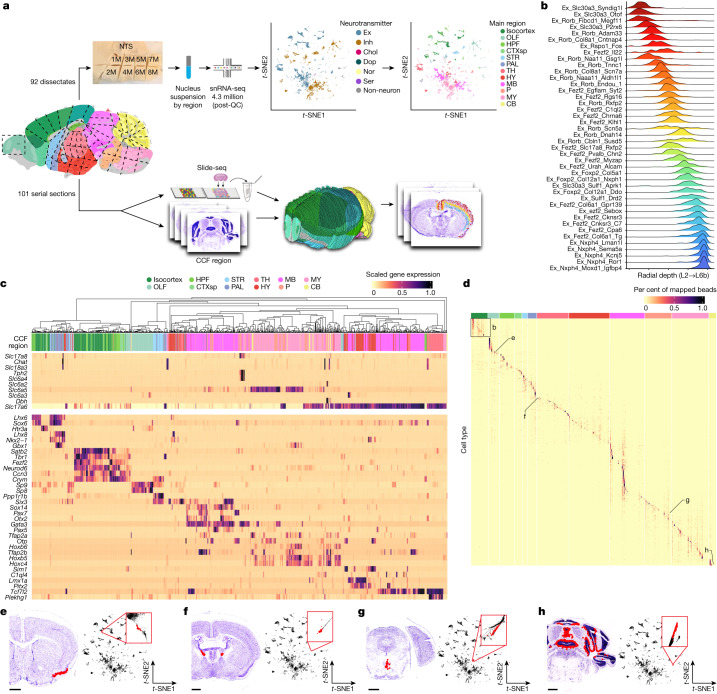
The function of the mammalian brain relies upon the specification and spatial positioning of diversely specialized cell types. Yet, the molecular identities of the cell types and their positions within individual anatomical structures remain incompletely known. To construct a comprehensive atlas of cell types in each brain structure, we paired high-throughput single-nucleus RNA sequencing with Slide-seq1,2-a recently developed spatial transcriptomics method with near-cellular resolution-across the entire mouse brain. Integration of these datasets revealed the cell type composition of each neuroanatomical structure. Cell type diversity was found to be remarkably high in the midbrain, hindbrain and hypothalamus, with most clusters requiring a combination of at least three discrete gene expression markers to uniquely define them. Using these data, we developed a framework for genetically accessing each cell type, comprehensively characterized neuropeptide and neurotransmitter signalling, elucidated region-specific specializations in activity-regulated gene expression and ascertained the heritability enrichment of neurological and psychiatric phenotypes. These data, available as an online resource ( www.BrainCellData.org ), should find diverse applications across neuroscience, including the construction of new genetic tools and the prioritization of specific cell types and circuits in the study of brain diseases.


Conflict of interest statement

F.C. and E.Z.M. are academic founders of Curio Bioscience.

Figures

Fig. 1
Fig. 1. Spatially mapping cell types using whole-brain snRNA-seq and Slide-seq datasets.
a, Schematic of the experimental and computational workflows both for whole-brain snRNA-seq sampling (upper arrows) and for Slide-seq sampling and CCF alignment (lower arrows). The t-distributed stochastic neighbour embedding (t-SNE) representations of gene expression relationships amongst 1.2 million spatially mapped snRNA-seq profiles (downsampled from 4.3 million) are coloured by neurotransmitter identity (upper left panel) and most common spatially mapped main region (upper right panel). Adapted from ref. , Allen Institute. b, Ridge plot depicting the spatial distributions of excitatory cortical cell types along the laminar depth of cortex (layers 2 to 6b) in the Slide-seq dataset. c, Heat maps depicting expression of the main neurotransmitter genes (upper panel) and canonical neuronal cell type markers (lower panel) across all 1,260 spatially mapped neuronal clusters. Cell types are annotated by the cluster dendrogram. d, Heat maps showing the spatial distributions of each spatially mapped cluster (rows) within each DeepCCF structure (columns; a complete list is in Supplementary Table 4). Example mapped cell types in other panels are labelled on the heat map. eh, Example confident mappings of neuronal cell types (confidence value > 0.3) (Methods) throughout the brain plotted in the CCF-aligned Slide-seq data (main plots) and in t-SNE space (insets) for the following cell types: Ex_Rorb_Ptpn20 (e, 35 arrays, 3,140 confident beads total), Ex_Ebf2_Iigp1_1 (f, two arrays, 84 confident beads total), SerEx_Fev_A2m (g, six arrays, 201 confident beads total), Inh_Nrk_Kctd16 (h, 25 arrays, 4,918 confident beads total). Scale bars, 1 mm. CB, cerebellum; CTXsp, cortical subplate; Chol, cholinergic neurons; Dop, dopaminergic neurons; Ex, excitatory neurons; HPF, hippocampal formation; HY, hypothalamus; Inh, inhibitory neurons; L, cortical layer; MB, midbrain; MY, medulla; NTS, nucleus tractus solitarii; Nor, noradrenergic neurons; OLF, olfactory areas; P, pons; PAL, pallidum; STR, striatum; Ser, serotonergic neurons; TH, thalamus; QC, quality control.
Fig. 2
Fig. 2. Variation in neuronal diversity across neuroanatomical structures.
a, Cumulative number of cell types needed to reach 95% of mapped beads in each DeepCCF region (right panel; defined in Supplementary Table 4) and averaged within individual main regions (left panel). The DeepCCF regions with the largest values are labelled. b, Force-directed graph showing cell type sharing relationships amongst DeepCCF regions. Edges are weighted by the Jaccard overlap between each region (Methods). c, Ridge plot depicting the transcriptomic distance from selected regions’ projection and interneuron cell types to their proximate neighbourhoods, separating each neighbourhood into their CCF regions (Methods). d, Example confident mappings of the nearest neighbour cell types (confidence value > 0.3) (Methods) for cerebellar interneurons grouped by excitatory and inhibitory index cell types. Inset highlights the neuroanatomical annotation of the dorsal cochlear nucleus from the Allen Mouse Reference Atlas. Adapted from ref., Allen Institute. Scale bars, 1 mm. CBN, cerebellar nuclei; CBX, cerebellar cortex; CNU, cerebral nuclei; HB, hindbrain; Isoctx, isocortex.
Fig. 3
Fig. 3. Neurotransmission and NP usage across regions of the mouse brain.
a, Upset plot of the frequency of neurotransmitter usage by individual snRNA-seq-defined cell types (upper panel). Dot plot depicting the spatial distribution of cell types in each of the neurotransmitter groups across major brain areas (lower panel). IB, interbrain. b, Point estimates of the fraction of each DeepCCF region composed of mapped inhibitory cell types. Data are presented as this calculated proportion (central dots) with the 95% confidence interval of the corresponding binomial distribution denoted by the error bars (Methods). c, Histograms denoting the number of distinct NPs (upper panel) and neuropeptide receptors (NPRs; lower panel) expressed in each snRNA-seq-defined neuronal cell type. d, Fraction of all cells expressing each NP (y axis) in each of the 12 main brain areas. Regions accounting for more than 50% of total expression of that NP are coloured and labelled. n = 43 NPs examined over 1,182 cell types. Box plots are centred at the median and bounded by the interquartile range (IQR; 25th–75th percentiles), with the lower whisker at the data point greater than or equal to (25th percentile − 1.5 × IQR) and the upper whisker at the data point less than or equal to (75th percentile + 1.5 × IQR). e, Dot plot depicting the number of cells expressing each NP (left of the dotted line) and NPR (right of the dotted line) within each major cell class. OPC, oligodendrocyte precursor.
Fig. 4
Fig. 4. Patterns of activity-dependent gene expression across brain regions.
a, Box plots quantifying mean core IEG Slide-seq counts per 10,000 coloured by main brain regions. n = 232 DeepCCF regions examined across 12 main regions. Box plots are centred at the median and bounded by the IQR (25th–75th percentiles), with the lower whisker at the data point greater than or equal to (25th percentile − 1.5 × IQR) and the upper whisker at the data point less than or equal to (75th percentile + 1.5 × IQR). b, Downsampled dot plot of correlation coefficients between Fos and candidate ARGs (columns) across major regions of the brain (rows). Genes are coloured by their established ARG gene set identity if applicable. Numbers at the bottom correspond to ARG cluster identities as determined by hierarchical clustering. PRG, primary response gene; SRG, secondary response gene. c, Scatterplot quantifying transcription factor enrichment (P < 0.05, FDR corrected) between excitatory and inhibitory populations. Enrichment scores are computed by fgsea using a positive one-tailed test. Transcription factors are coloured by their cell type enrichment specificity.
Fig. 5
Fig. 5. Heritability enrichment for traits studied by GWAS across brain cell types.
a, Bar plots quantifying significantly enriched (P < 0.05, computed by single-cell disease relevance score (scDRS) using the one-sided Monte Carlo test, FDR corrected) (Methods) cell types for each trait in non-neurons (grey) and neurons (coloured by main region). b, FDR-adjusted (adj.) −log10 P value enrichment scores for each cell type, grouped and coloured by their main regions, for schizophrenia. Squares and triangles denote excitatory and inhibitory clusters, respectively; glia are shown in grey on the far right. P values are computed by scDRS using a one-sided Monte Carlo test. c, Ridge plots showing the layer distribution of each excitatory cortical cell type found to be significantly enriched (P < 0.05, computed by scDRS using the one-sided Monte Carlo test, FDR corrected) for schizophrenia heritability. d, Dot plot of expression of markers of striatal SPN subtype identity grouped by category (overall cell class identity, pathway identity, matrix versus striosome and eSPN identity). Six additional genes that are enriched in the schizophrenia-enriched (P < 0.05, computed by scDRS using the one-sided Monte Carlo test, FDR corrected) SPN types are also shown. STRd, striatum dorsal region; STRv, striatum ventral region; SCZ, schizophrenia. e, Representative sections showing the confident mappings of three SPN cell types (confidence value > 0.3) (Methods) significantly enriched (P < 0.05, computed by scDRS using the one-sided Monte Carlo test, FDR corrected) for schizophrenia heritability exemplifying Inh_Ppp1r1b_Drd2_Sema5d_2 (top panel; 9 arrays, 178 confident beads total), Inh_Ppp1r1b_Drd2_Sema5d_1 (middle panel; 6 arrays, 119 confident beads total), and Inh_Ppp1r1b_Drd1_Zp3r_4 (bottom panel; 19 arrays, 1,008 confident beads total). Scale bars, 1 mm.
Extended Data Fig. 1
Extended Data Fig. 1. Quality control and summary statistics of the snRNA-seq analysis.
a, Sankey diagrams showing the number of nuclei (top) and clusters (bottom) retained and removed at each step of our quality control workflow. The final retained numbers include immune cells. mt (mitochondrial gene). b, Stacked bar plots showing the nuclei sampled per region, for each animal replicate. Female donor IDs contain an “F”, while male donors contain an “M”. The top colouring indicates the dissectate’s major region. c, Bar plots showing the average UMIs per nucleus in each dissectate, coloured by main region. Error bars indicate standard error of each dissectate’s average number of UMIs. n = 4388420 nuclei examined over 92 dissectates. d, Violin plots showing the log10 distribution of the UMIs per nucleus in each major cell class (including immune cell classes). n = 4407296 nuclei examined over 16 cell classes. Box plots centred at median, bounded by IQR (25-75th percentile), with lower whisker at data point >= (25th percentile − 1.5*IQR) and upper whisker at data point <= (75th percentile + 1.5*IQR). e, Stacked bar plots of the nuclei sampled in each major mouse brain region, sub-setted by individual dissectate. f, Histogram of the maximal proportional representation of individual dissectates in each snRNA-seq cluster. g, Heatmap representing a confusion matrix between clustering of the snRNA-seq data in the current study (x-axis), and published studies (y-axis), for the mouse motor cortex (left) and cerebellum (right). h, Histogram of the log10 nuclei recovered from each major cell class (including immune cell classes). i, Plot indicating the probability of sampling 19 very rare populations (prevalence 0.0024% among all mapped cell types) as a function of the total number of mapped cells profiled in experiment (probability estimation in Methods). Number of high-quality nuclei profiled here (4388420) and corresponding probability are indicated.
Extended Data Fig. 2
Extended Data Fig. 2. Quality control and summary statistics of CCF integration and cell type mapping.
a, Example images of adjacent Nissl sections aligned to CCF with 2D rigid transformation (wireframe outline) before (left) and after (right) correcting alignment with a 2D diffeomorphism. Red arrows point to example regions with incorrect alignment, and improvement after application of the correction. b, Expression of three highly specific marker genes that label the ventricular lining (Tmem212; 309 beads with non-zero expression), dentate gyrus granule layer (Dsp; 318 beads with non-zero expression), and layer 6b of isocortex (Ccn2; 418 beads with non-zero expression) in Slide-seq (top row); scale bar, 1 mm. Bottom row shows the positions of individual beads with expression with respect to the boundaries of the expected CCF region (purple). c, Density plot of the distance of each bead expressing each of the three marker genes (or all combined) shown in b across the corresponding Slide-seq sections. The full width half maximum of the density profile is shown. d, Heatmap representing the frequency of bead mappings for each glial cell type, across DeepCCF regions. e, Visualization of cell type dendrogram where each cluster (leaf of the tree) is coloured by their CCF region localization. The outer ring displays the boundaries of the 223 metaclusters where the alternating colours signify transitions between groups.
Extended Data Fig. 3
Extended Data Fig. 3. Extended analyses quantifying neuronal cell type diversity across brain areas.
a, Heatmap representing the weighted Jaccard similarity in cell type composition between each of the 12 main brain areas (Methods). b, Histogram of the minimum number of genes required to uniquely define each cell type across the nervous system. The algorithm was repeated, tolerating genes to be the same amongst different numbers of nearest cluster neighbours. c, Cumulative distribution plots of the number of genes needed to label each cell type, within each of the 12 major brain areas. Within each region, each of the sets of individually coloured plots denotes an algorithmic run with a different number of nearest neighbours that are tolerated as having the same gene markers (absolute number in parentheses at right). The coloured percentages denote the proportion of cell types for which the algorithm was able to find a solution. d, Bar plot quantifying the significantly enriched GO terms using EnrichR (hypergeometric test, p-adj <0.05) in the minimum-sized collated gene list after hierarchical reduction (Methods), coloured by the absolute number of genes related.
Extended Data Fig. 4
Extended Data Fig. 4. Extended analyses of projection and interneuron cell type relationships across regions.
a, Normalized gene expression heatmaps of the neighbouring cell types for clusters within each metacluster. The clusters are sorted by increasing distance to the index metacluster (nearest at top), with the dotted horizontal line delineating the proximate neighbourhood (Methods). Marker genes are plotted to show the calibration of neighbourhoods to include only similar cell types. b, Extended ridge plots depicting the transcriptomic distance from selected regions’ projection and interneuron cell types to their proximate neighbourhoods, separating each neighbourhood into their CCF regions (Methods). The neurons are split into the relevant metacluster for each region.
Extended Data Fig. 5
Extended Data Fig. 5. Extended analyses of neurotransmitter and neuropeptide usage across the brain.
a, Stacked bar plots of the number of cell types with confident mappings in each deep CCF region (conf. value > 0.3, Methods), sub-setted by neurotransmitter group. Deep CCF regions are coloured on the left by their corresponding major brain region. b, Representative sections showing the confident mappings of all cell types within three neurotransmitter groups (conf. value > 0.3, Methods). c, Violin plots of the number of neuropeptides expressed in each cluster, stratified by main brain region. d, Dot plot showing scaled Slide-seq counts per 10,000 of ligand-receptor pairs across main brain regions.
Extended Data Fig. 6
Extended Data Fig. 6. Extended analyses related to activity-related genes.
a, Comparison of correlations (right) and quantile of correlation (left) between each gene and both Fos (x-axis) and Junb. Red dots indicate the genes that were selected as candidate ARGs. b, Scatter plot quantifying the node degree of each gene in the activity-regulated gene network. Genes labelled in red were selected as our core IEGs (Methods). c, Bar plots showing the average Slide-seq counts per 10,000 of the core IEG metagene (the eight genes highlighted in panel b). Error bars indicate standard error of average counts per deep CCF region and dashed black lines indicate average counts per main brain region. d, Scaled mean expression of the core IEGs, within each main region, separated by neurotransmitter group. e, Extended dot plot of correlation coefficients between Fos and candidate ARGs (columns) across major regions of the brain (rows). Genes are coloured by their established ARG gene set identity, if applicable. Numbers at the bottom correspond to ARG cluster identities as determined by hierarchical clustering. f, Enrichment analysis of each candidate ARG cluster with three established ARG gene sets. P-values were computed from Fisher’s exact test using GeneOverlap and Bonferroni-corrected for multiple hypothesis testing (Methods). Dotted red line indicates an adjusted p-value threshold of 0.05.
Extended Data Fig. 7
Extended Data Fig. 7. Extended analyses of heritability enrichment in murine brain cell types.
a, Correlation plot of p-value enrichment scores (one-sided MC test from scDRS, FDR-corrected, Methods) for each cell type across different scDRS settings: A) default parameters (Methods) B) MAGMA gene z-score > 2.5, C) control gene set size of 2,000, D) control gene set size of 500, E) input expression dataset at the single-cell level (versus pseudocells), F) adjust for cell type proportions. b, FDR-adjusted -log10 p-value enrichment scores for each cell type, grouped and coloured by main region, for an extended set of GWAS-measured traits. Squares and triangles denote excitatory and inhibitory clusters, respectively; glia are shown in grey on the far right of each plot. P-values computed by scDRS using a one-sided MC test. c, Dot plot of the expression of key cortical pyramidal cell type markers within the eight isocortical clusters that were significantly enriched (p-value < 0.05, computed by scDRS using one-sided MC test, FDR-corrected) for schizophrenia heritability.

References

    1. Rodriques SG, et al. Slide-seq: a scalable technology for measuring genome-wide expression at high spatial resolution. Science. 2019;363:1463–1467. doi: 10.1126/science.aaw1219. - DOI - PMC - PubMed
    1. Stickels RR, et al. Highly sensitive spatial transcriptomics at near-cellular resolution with Slide-seqV2. Nat. Biotechnol. 2021;39:313–319. doi: 10.1038/s41587-020-0739-1. - DOI - PMC - PubMed
    1. Zeng H. What is a cell type and how to define it? Cell. 2022;185:2739–2755. doi: 10.1016/j.cell.2022.06.031. - DOI - PMC - PubMed
    1. Zeng H, Sanes JR. Neuronal cell-type classification: challenges, opportunities and the path forward. Nat. Rev. Neurosci. 2017;18:530–546. doi: 10.1038/nrn.2017.85. - DOI - PubMed
    1. Wang Q, et al. The Allen Mouse Brain Common Coordinate Framework: a 3D reference atlas. Cell. 2020;181:936–953.e20. doi: 10.1016/j.cell.2020.04.007. - DOI - PMC - PubMed

Publication types