Single-cell analysis of chromatin accessibility in the adult mouse brain

Abstract

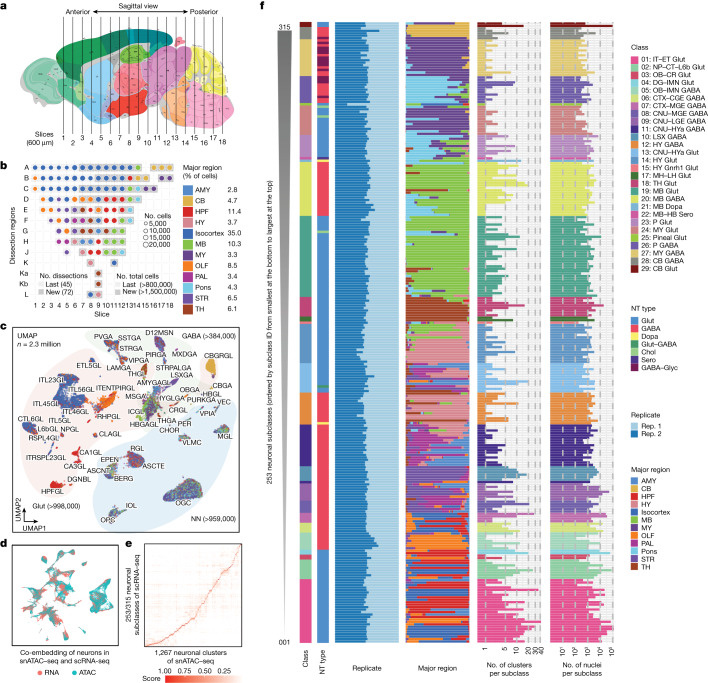
Recent advances in single-cell technologies have led to the discovery of thousands of brain cell types; however, our understanding of the gene regulatory programs in these cell types is far from complete^1-4. Here we report a comprehensive atlas of candidate cis-regulatory DNA elements (cCREs) in the adult mouse brain, generated by analysing chromatin accessibility in 2.3 million individual brain cells from 117 anatomical dissections. The atlas includes approximately 1 million cCREs and their chromatin accessibility across 1,482 distinct brain cell populations, adding over 446,000 cCREs to the most recent such annotation in the mouse genome. The mouse brain cCREs are moderately conserved in the human brain. The mouse-specific cCREs-specifically, those identified from a subset of cortical excitatory neurons-are strongly enriched for transposable elements, suggesting a potential role for transposable elements in the emergence of new regulatory programs and neuronal diversity. Finally, we infer the gene regulatory networks in over 260 subclasses of mouse brain cells and develop deep-learning models to predict the activities of gene regulatory elements in different brain cell types from the DNA sequence alone. Our results provide a resource for the analysis of cell-type-specific gene regulation programs in both mouse and human brains.

Fig. 1. Single-cell analysis of chromatin accessibility in the adult whole mouse brain.

a, Schematic of the sample dissection strategy. The brain map was generated using coordinates from the Allen Mouse Brain Common Coordinate Framework (CCF) v.3 (ref. ). b, The number of nuclei for 117 dissections after quality control and doublet removal. The dot size is proportional to the size of cells and the dissections that were not covered by our previous study are shown in grey. A to L on the left were used as the dissection region labels on each slice (details are provided in Extended Data Fig. 1). The number of dissections represents the number of dissections covered by our previous study (last) and updated in the current study (new). The total number of cells represents the number of cells covered by our previous study (last) and updated in the current study (new). c, UMAP embedding and clustering analysis of snATAC–seq data. The light colours denote major cell classes. NN, non-neuronal cells. Cells are coloured on the basis of major regions as in b. d, The co-embedding UMAP embedding of the neuronal cells from scRNA-seq data and the snATAC–seq data on the same space coloured by the two modalities. e, The consensus score between neuronal subclasses from the scRNA-seq data above and L4-level neuronal clusters from our snATAC–seq data. f, The 253 neuronal subclasses in our snATAC–seq data matched to neuronal subclasses in the scRNA-seq above, and ordered on the basis of the subclass IDs (for all of the following figures, the order was kept the same unless otherwise mentioned). From left to right, the bar plots represent the class, major neurotransmitter (NT) type, biological replicate distribution of nuclei, major region distribution of nuclei, number of clusters and number of nuclei. Detailed information about class, neurotransmitter type and subclass is reported in the companion paper. A list of full names of the subclasses is provided in Supplementary Table 3. CTX, cerebral cortex; HYa, anterior hypothalamus; L6b, layer 6b; LSX, lateral septal complex; IT, intratelencephalic; ET, extratelencephalic; NP, near-projecting; CT, corticothalamic; OB, olfactory bulb; CR, Cajal-Retzius; DG, dentate gyrus; IMN, immature neurons; CGE, caudal ganglionic eminence; MGE, medial ganglionic eminence; CNU, cerebral nuclei; LGE, lateral ganglioniceminence; MH, medial habenula; LH, lateral habenula; Chol, cholinergic neurons; Dopa, dopaminergic neurons; Glyc, glycinergic neurons; Sero, serotonergic neurons.

Fig. 2. Identification and characterization of cCREs across mouse brain cell types.

a, The fraction of cCREs that overlaps with annotated sequences in the mouse genome was determined using HOMER. TTS, transcription termination site; UTR, untranslated region. b, The overlaps between the cCREs in this study (red) and the representative DHSs (rDHSs; blue) from the SCREEN database. c, The average PhastCons conservation scores of cCREs (red) overlapping (ovlp) with rDHSs, cCREs (blue) with no overlaps with rDHSs, and random genomic background (grey) were determined using deepTools. d, The fraction of cCREs captured by different cell subtypes for peak calling. Left, the cCREs with no overlaps with rDHSs. Right, the cCREs with overlaps with rDHSs. e, Genome browser tracks of the two types of cCREs. Left, cCREs with no overlaps with rDHSs. Right, the cCREs with overlaps with rDHSs. The subclass names were the same as for the scRNA-seq data in the companion paper. f, The chromatin accessibility at 150 cis-regulatory modules across the 244 shared cell subclasses in the snATAC–seq data for all of the 1 million cCREs (top left). Rows represent subclasses, and columns are representative cCREs sampled from each module. Right, heat map showing the snDNA-methylation signals from the snmC-seq analysis at the genomic locations of the corresponding cCREs for the same subclasses. Bottom, heat maps similar to those above but for only the 460,000 cCREs with no overlaps with the ENCODE rDHSs.

Fig. 3. Integrative analysis to identify the potential enhancer–gene connections across the whole mouse brain.

a, Schematic of the computational strategy used to identify cCREs that are positively correlated with the mRNA expression of the target genes; PCCs were calculated across 275 cell subclasses between the snATAC–seq and scRNA-seq data. Co-accessible cis-regulatory DNA interactions were predicted using Cicero for each cell subclass. b, In total, 613,485 pairs (red) of positively correlated cCRE–gene pairs were identified (FDR < 0.01). The grey-filled curve shows the distribution of PCCs for randomly shuffled cCRE–gene pairs. c, The chromatin accessibility of putative enhancers (left); mRNA expression of the linked genes in the 275 cell subclasses across the whole mouse brain (middle); and the enrichment of known TF motifs in distinct enhancer gene modules (right). A total of 428 out of 440 known motifs from HOMER with enrichment P < 10⁻¹⁰ is shown. The unadjusted P values were calculated using two-sided Fisher’s exact tests.

Fig. 4. Inference of subclass-specific GRNs across the whole mouse brain.

a, Example of the GRN inferred in telencephalon-region astrocyte (ASC-TE_NN) using CellOracle. Edges are weighted and directed to reflect the putative regulation strength and mode (inhibition or activation). b, The degree distribution of the GRN in a. P(k), the probability of a node having k degree in the GRN. The degree of one node is the number of other nodes with links to it. c, The number of TFs, the number of genes, the number of regulated TFs per gene and the number of genes regulated by the TFs among the GRNs for each of 267 cell subclasses. The numbers of dots in each box plot from left to right are as follows: 267, 267, 185,000 and 82,000. For the latter two plots, treat TFs and genes from different subclasses as different ones. For the box plots in c, the box limits span the first to third quartiles, the centre line denotes the median and the whiskers show 1.5× the interquartile range. d, Normalized histograms of the number of the regulated double-positive network motifs for each main cell class. The lines are the kernel-based density curves fitted for different histograms. e, Histograms of the two network motifs for five mouse brain regions: telencephalon (isocortex, OLF, HPF, STR, PAL and AMY), diencephalon (TH and HY), MB, hindbrain (MY and pons) and CB. f, Heat map of eigenvector-based centralities or importance scores of TFs in each of the subclass-specific GRNs. Each row represents a TF, and each column a subclass. The orders of the TFs and subclasses are based on the companion paper for the similar heat map but using the scRNA-seq data. The names of the rows and columns are listed in Supplementary Table 18.

Fig. 5. Analyses of chromatin accessibility at TEs of cCREs.

a, Schematic of mouse-specific and orthologous cCREs. The bar plot shows the numbers of mouse-specific and orthologous cCREs. b, The fraction of the genomic distribution of mouse-specific and orthologous cCREs. c, The fraction of cCREs overlapping with TEs in each subclass of Glut neurons, GABAergic neurons, dopaminergic neurons, cholinergic neurons, serotonergic neurons, glycinergic neurons and non-neurons. The two curves show the Gaussian distribution from the mixture model. highTE-Glut refers to the Glut neuron subclasses with a high percentage of their cCREs overlapping with TEs. d, Gene Ontology (GO) analysis revealing an enrichment of neuronal-specific functions among genes that exhibited positive correlations with TE-cCREs (TE-related cCREs) in highTE-Glut subclasses, compared with genes positively correlated with TE-cCREs in all subclasses. e, GO analysis revealing an enrichment of neuronal-specific functions among genes that exhibited positive correlations with TE-cCREs in highTE-Glut subclasses, compared with genes positively correlated with all cCREs in highTE-Glut subclasses. f, DCA at TE-cCREs in highTE-Glut subclasses compared with other subclasses. The top ten DCA TE-cCREs correlating with synaptic-related genes are shown. The top ten DCA TE-cCRE–gene pairs (such as L1MB8–Cdkl5) are indicated by red boxes. The super family of the top ten DCA TE-cCREs are indicated by different shapes. g, The top three motif families enriched in the DCA TE-cCREs in highTE-Glut neurons. The unadjusted P values were calculated using two-sided Fisher’s exact tests. h, Genome browser tracks of aggregate chromatin accessibility profiles for NN, GABA, highTE-Glut and other Glut subclasses at selected DCA TE-cCREs and gene pairs. RNA signals shown here were collected from the previous study. PDC, proximal–distal connections.

Fig. 6. Deep-learning models predict chromatin accessibility in different brain cell types from the DNA sequence.

a, Schematic of the deep-learning (DL) model Basenji for predicting chromatin accessibly. b, The number of subclasses of each cell class in the training dataset. c, The accuracy (Pearson correlation) of each class. n = 93 (GABA), n = 111 (Glut) and n = 17 (NN) subclasses. d, The AUROC was calculated for representative subclasses by comparing the peaks called from predicted genomic signals with the peaks called from real experimental signals. e, The model’s ability to predict cell-type-specific patterns of open chromatin. The coefficient of variance (variance/mean) across cell types was compared with the Pearson r calculated between true signals and the predicted signals across cell subclasses. Each dot represents one cCRE in the testing set. f, True signals from ATAC–seq data in mouse cell subclasses were compared with the predicted chromatin accessibility in the test set. Representative loci near Nr4a2, Pou4f2, Ecel1, Hopx, Apoe and Pf4 are shown. g, Schematic of predicting potential chromatin accessibility signals using human DNA sequence as inputs. h, The AUROC was calculated for matched human cell types. n = 26 cell types for the human brain dataset. i, The Pearson r of true signals and the predicted signals across cell types for all tested cCREs, tested distal cCREs and tested proximal cCREs. The numbers of overall, distal and proximal cCREs are 452,531, 437,207 and 15,324, respectively. j, True signals captured from ATAC–seq analysis in human cell types and predicted chromatin accessibilities are shown at representative genomic loci near the genes CUX2, GAD2, DRD1 and OLIG1. Cell-type-specific cCREs are highlighted in grey. For the box plots, the box limits span the first to third quartiles, the centre line denotes the median and the whiskers show 1.5× the interquartile range.

Extended Data Fig. 1. Maps of the 117 anatomical dissections of the adult whole mouse brain.

a, Schematic of brain tissue dissection strategy. Mouse brains were cut into 600-µm-thick coronal slices. b, These brain maps were generated using coordinates from the Allen Mouse Brain Common Coordinate Framework (CCF) v3 (ref. ). Brain regions dissected from each coronal slice are marked according to the Allen Brain Reference Atlas. The frontal view of each slice from slices 1–18 is shown, with the dissected regions alphabetically labelled on the left, and the anatomic labelling listed on the right. A detailed list of the dissected regions and the full anatomic labelling can be found in Supplementary Table 1.

Extended Data Fig. 2. Quality control metrics of the snATAC-seq datasets at the bulk level.

a, Box plots showing the distribution of mapping ratios (the fraction of the mapped sequencing reads) in replicates (rep) 1 and 2 of the snATAC-seq experiments from each brain dissection. b, Box plots showing the distribution of the number of proper read pairs (reads are correctly oriented) in rep 1 and 2 of the snATAC-seq experiments. c, Box plots showing the distribution of numbers of unique chromatin fragments detected in rep 1 and 2 of the snATAC-seq experiments. d, Box plots showing the distribution of the number of unique barcodes captured in replicates 1 and 2 of snATAC-seq experiments. In a-d, the number per each boxplot (rep1 or rep2) is 117. In each boxplot, the box spans the first to third quartiles, the horizontal line denotes the median, and whiskers show 1.5x the interquartile range. e, Frequency distribution plot showing the fragment size distribution of each snATAC-seq sample or datasets (234 samples/datasets in total). f, Heat map showing the pairwise Spearman correlation coefficients of the mapping correlations of the bam files between the snATAC-seq datasets. The column and row names consist of two parts: brain region name and replicate label. Study represents dissections covered by our previous study (Last) or updated in the current study (New).

Extended Data Fig. 3. Quality control metrics of the snATAC-seq datasets at the single-cell level.

a, Dot plot illustrating fragments per nucleus and individual TSS enrichment. Nuclei in the top right quadrant were selected for analysis (TSS enrichment > 10 and > 1,000 fragments per nucleus). b, Box plots showing the AUPRCs of AMULET and Scrublet on the simulated data sets from the corresponding samples labelled in x axis. Each bar represents the mean value of 10 random experiments with 1x standard deviation as the error bar. Two-sided t-tests were used, and *** means P-value < 0.0001. c. Box plots showing the doublet rates across the samples. Samples were grouped based on their replicate information. n = 117 biologically independent samples for each replicate 1 and 2. d, Number of nuclei retained after each step of quality control. e, Bar plots showing the numbers of nuclei passing quality control for subregions. f, Box plots showing the TSS enrichments and unique fragments per nuclei for the replicates in different mouse brain regions. The smallest sample size is ORB region replicate 1 with n = 4,943 cells, while the largest is PAL-2 replicate 1 with n = 12,464 cells. In c and f, boxes span the first to third quartiles, horizontal line denotes the median, and whiskers show 1.5x the interquartile range.

Extended Data Fig. 4. Iterative clustering for the snATAC-seq data.

a, A multi-stage cell clustering pipeline is organized for all the nuclei passing our quality control. b, Violin plots showing the number of unique fragments per nucleus in each cell subclass. c, Violin plots showing the TSS enrichment in each nucleus of each cell subclass. d, Boxplots of acceptance rates from k-nearest neighbour batch effect test (kBET) for the 275 subclasses. Boxes span the first to third quartiles, horizontal line denotes the median, and whiskers show 1.5× the interquartile range. Two-sided t-tests showed no significant P-values between the values from the two boxes. e, Distribution of the local inverse Simpson’s index (LISI) scores for cells in each subclass.

Extended Data Fig. 5. Quality and reproducibility of the cell clusters.

a, CDF plot showing the consistency of the estimated fraction of each cell subclass between the biological replicates. Two-sided Kolmogorov-Smirnov test shows no significant difference between the biological replicates. b, Box plots of the P values of two-sided Kolmogorov-Smirnov tests illustrate consistent results between the two biological replicates for each subclass across major brain regions, sub-regions and brain dissections tested. n = 12 comparisons for major regions, n = 41 comparisons for sub-regions and n = 117 comparisons for dissection regions. c, Heat map showing the pairwise Spearman correlation coefficients of cell subclass composition between each replicate of brain dissections. The column and row names consist of two parts: brain region name and replicate label. For example, CB-1.1 represents the replicate 1 of the first brain dissection of the cerebellum (CB-1). The embedded box plot shows the distribution of Spearman correlation coefficients between two biological replicates, replicates from intra-major brain regions and inter-major brain regions. Significance is denoted as ***P < 2.2e-16, determined by one-sided Wilcoxon rank-sum test. n = 22720 pairs for “intra-major regions” group, n = 4424 pairs for “inter-major regions” group, n = 117 for “between replicates” group. Boxes span the first to third quartiles, horizontal line denotes the median, and whiskers show 1.5x the interquartile range.

Extended Data Fig. 6. Integration analysis between the snATAC-seq and the scRNA-seq data for neurons and non-neurons separately.

UMAP on the co-embedding space of neurons from the snATAC-seq data (a) and scRNA-seq data (b). Colours as major regions. c, The co-embedding UMAP embedding of non-neuronal cells from the scRNA-seq data and the snATAC-seq data on the same space coloured by the two modalities. UMAP on the co-embedding space of non-neurons from snATAC-seq data (d) and scRNA-seq data (e). Colours as major regions. f, Consensus scores (i.e., transfer-label scores) between non-neuronal subclasses from the scRNA-seq data and L4-level non-neuronal clusters from the snATAC-seq data. g, Consensus scores between neuronal clusters from the scRNA-seq data of Allen Institute and L4-level neuronal clusters from the snATAC-seq data. h, Consensus score between non-neuronal clusters from the scRNA-seq data and L4-level non-neuronal clusters from the snATAC-seq data. i, The 22 non-neuronal subclasses matched to the non-neuronal subclasses in the scRNA-seq. From left to right, the bar plots represent class, biological replicate distribution of nuclei, major region distribution of nuclei, number of clusters, and number of nuclei.

Extended Data Fig. 7. Marker genes for the subclasses after integration in the snATAC-seq data using the imputed gene expressions.

Dotplot showing the snATAC-seq gene activity scores of the marker genes (columns) used for identification of the scRNA-seq data across the cell subclasses. The first 13 columns correspond to major neuronal cell type marker genes including neurotransmitter genes as follows: Snap25 (Neuron), Gad1 (GABA), Gad2 (GABA), Slc32a1 (GABA), Slc17a6 (Glut-subcortical), Slc17a7 (Glut-cortical), Slc17a8 (Glut), Slc6a5 (Gly-GABA), Slc6a4 (Glut-Sero), Slc6a3 (Dopa), Slc18a3 (Chol), Hdc (Hist), Slc6a2 (Nora). The subsequent columns are the most occurring marker gene reported within each Allen Institute subclass designation corresponding to each subclass annotation (row) of the snATAC-seq data.

Extended Data Fig. 8. Cellular composition of brain dissections for cell subclasses.

a, Bar plot shows the total number of nuclei sampled for each brain dissection region. b, Normalized percentages (pct) of each subclass in all the dissected regions are shown as different sized dots. The sizes of dots correspond to the percentage and the colours of the dots indicate the brain dissections.

Extended Data Fig. 9. Statistics of peak calling on snATAC-seq data for each cell subtype.

a, Schematic of peak calling and filtering pipeline. b, Density distribution plot showing the fraction of cells per cell type in which a peak was accessible and a corresponding background for each cell type. For each cell type, the background is defined as the non-DHS and non-peak regions randomly picked from the genome. c, Venn plot showing the overlapping between the peaks from the whole mouse brain and the ones from the cerebral regions. d, Enrichment analysis of the peak sets with a 15-state ChromHMM model in the mouse brain chromatin. e, Density map comparing the median and maximum variation of chromatin accessibility at each cCRE across cell subclasses. The left density map refers to the cCREs overlapping with the ENCODE DHSs, and the right one refers to the cCREs having no overlaps with the ENCODE DHSs. i, Scatter plot showing entropy (blue) and sparseness (red) trends when increasing the number of modules used for non-negative matrix factorization. When the module number is 150, we can see a significant drop in entropy and a significant increase in sparseness. j, The red arrows point to the two subclasses with lowest number of cells in the snmC-seq data.

Extended Data Fig. 10. Characterization of predicted cCRE-target gene pairs.

a, Scatter plot showing the number of identified connections between all the cCREs pairs within 500k bp along with the number of nuclei for each cell subclass identified based on the integration analysis. b, Scatter plot showing the number of proximal-distal cCREs along with the number of nuclei for each cell subclass. c, Histogram showing the distances along the genome for each proximal-distal cCREs. d, Histogram showing the distances along the genome for each pair of enhancer and targeted gene’s promoter (positive proximal-distal cCREs) inferred by the correlation study (Fig. 3b). e, In total, 613,485 positively correlated proximal-distal cCREs and 107,413 negatively correlated proximal-distal cCREs were identified. f, Boxplot showing the identified potential enhancers for each of 20,703 gene in the positively correlated pairs. g, Boxplots of the enrichment scores (1 kb resolution) of aggregate peak analysis (APA) for the top 20% positive proximal-distal connections (ppdc) from several represented subclasses. Match, the subclass’s Hi-C data used for the same subclasses. Unmatch, the subclass’s Hi-C data used for other subclasses as a random background. 11 data points were included in the match group and 110 points in the unmatched groups. P value was calculated by the one-sided Wilcoxon rank sum test. In f and g, boxes span the first to third quartiles, horizontal line denotes the median, and whiskers show 1.5x (f) and 2x (g) the interquartile ranges. h. Heatmaps of enrichment signals for the top 10% global proximal-distal connections (pdc) and enrichment signals for the random pairs.

Extended Data Fig. 11. Inference of gene regulatory networks (GRNs) at cell subclass level across the whole mouse brain.

a, Schematic of identifying co-accessible cCREs for each cell subclass using Cicero. b, Schematic view of inference of GRNs from predicting the putative target genes’ expression with the corresponding transcription factors (TFs) for each cell subclass using CellOracle. c, Boxplot of 267 P values from two-sided Kolmogorov-Smirnov test to check power-law distributions of the nodes’ degrees from GRNs. Only one cell subclass (OB_Eomes_Ms4a15_Glut) did not pass this examination with the P values smaller than 0.05. The box spans the first to third quartiles, the horizontal line denotes the median, and whiskers show 1.5x the interquartile range. d, 15 commonly used network motifs used in our analysis. Each node is a TF or a gene, and edges describe the regulation directions, i.e., arrows pointed to the ones that were regulated by the source nodes or TFs. The blue colour means the negative regulation (TFs inhibit target gene expressions), while the orange colour means the positive regulation (TFs upregulate target gene expressions). PFL, positive-feedback loops; RDP, regulated double-positive; FC, fully connected triad; FFL, feedforward loops. SIM, single-input module. e, Stacked bar plots of the ratio of the network motifs above in each subclass. Each column responds to one cell subclass.

Extended Data Fig. 12. Histograms of the counts of the network motifs in each subclass’s gene regulation network (GRN) grouped by main class (a) or regions (b).

The names of the network motifs are the same ones in Extended Data Fig. 11d. Only the class with at least 3 subclasses were shown here. For each histogram, we added the corresponding density plot. The telencephalon region includes isocortex, olfactory bulb, hippocampus, striatum, pallidum, and amygdala; the diencephalon region includes thalamus and hypothalamus; the hindbrain includes pons and medulla. c, Normalized signals of Atf3 ChIP-seq at Klf4 in bone marrow-derived macrophages (BMM) showing Klf4 is likely to be a putative target of Atf3. d, Normalized signals of Atf3 ChIP-seq at Tal1 in bone marrow-derived macrophages (BMM) showing Tal1 is likely to be a putative target of Atf3.

Extended Data Fig. 13. Comparison of chromatin accessibility (CA) conserved and divergent cCREs between mouse and human.

a, A schematic of CA conserved and divergent cCREs. The CA-conserved cCREs are the cCREs in our snATAC-seq data that are conserved across species and have open chromatin in orthologous regions. The CA divergent cCREs are sequence conserved to orthologous regions but have not been identified as open chromatin regions in other species. The bar plot shows the numbers of CA-conserved and CA-divergent cCREs. b, Bar plot showing the relative fraction of CA conserved and divergent cCREs across subclasses. c, Radar chart showing the fraction of genomic distribution of CA-conserved and CA-divergent cCREs. The CA-conserved cCREs show an increase in percentage in Promoter-TSS regions. d, Histograms showing the number of CA-conserved and CA-divergent cCREs in subclasses. The number of CA-conserved cCREs is higher than CA-divergent cCREs. e, Histograms showing the CA-conserved cCREs captured by the number of cell subclasses. A fraction of CA-conserved cCREs are captured by more than 200 cell subclasses. f, Histograms showing the CA-divergent cCREs captured by the number of cell subclasses. Most CA-divergent cCREs are captured by less than 50 cell subclasses.

Extended Data Fig. 14. Analyses of chromatin accessibility at transposon elements (TEs) of cCREs.

a, Pie charts showing the genomic distribution of mouse-specific cCREs. b, Histograms showing the fraction of cCREs overlap with TEs in subclasses of glutamatergic neurons (Glut), non-glutamatergic neurons (nonGlut-Neu), and non-neurons (NN). c, Boxplot showing the fraction of cCREs overlap with TEs in highTE-Glut, other-Glut, nonGlut-Neu, and NN subclasses. The P values are calculated by the one-sided Wilcoxon rank-sum test. Boxes span the first to third quartiles, horizontal line denotes the median, and whiskers show 1.5× the interquartile range. There are n = 22 subclasses in the “highTE-Glut” group, n = 108 subclasses in the “other-Glut” group, n = 123 subclasses in the “nonGlut-Neu” group, and n = 22 subclasses in the “NN” group. d, Heatmap showing the fraction of genomic distribution of cCREs in each cell subclass. e, Heatmap showing the fraction of TE family distribution of cCREs in each cell subclass. f, GO analysis showing genes near TE-cCREs in highTE-Glut versus genes near TE-cCREs in all subclasses are enriched for neuronal specific functions. g, GO analysis showing genes near TE-cCREs in highTE-Glut versus genes near all cCREs in highTE-Glut are enriched for neuronal specific functions. h, Top3 motif families enriched in the TE-cCREs in highTE-Glut. The unadjusted P-values were calculated using a two-sided Fisher’s exact test. i, Top3 motif families enriched in the TE-cCREs which showed positively correlated with genes and occurred in highTE-Glut. The unadjusted P-values were calculated using a two-sided Fisher’s exact test. j, Volcano plot showing differential chromatin accessibility (DCA) TE-cCREs in highTE-Glut subclasses compared to other subclasses. The red colour labelled all DCA TE-cCREs which correlated with synaptic related genes. k, Genome browser tracks of aggregate chromatin accessibility profiles for NN, GABA, highTE-Glut, and other Glut subclasses at selected DCA TE-cCREs and gene pairs. RNA signals shown here were collected from previous study.

Extended Data Fig. 15. Accessible variability at transposon elements (TEs) across cell subclasses.

a, Density scatter plot comparing the averaged accessibility and coefficient of variation across cell subclasses at each transposon element. Variable TEs are defined on the upper right side of dash lines, invariable TEs are defined on the upper left of dash lines. b, Normalized accessibility at variable TEs in different cell subclasses. The middle bar plot showing correlation between mCG level and accessibility at variable TEs across subclasses. The right bar plot shows correlation between expression level and accessibility at variable TEs across subclasses. c, Top10 motifs enrich in positively distal cCREs overlapped with variable TEs. The unadjusted P-values were calculated using a two-sided Fisher’s exact test. d, Normalized accessibility at invariable TEs in different cell subclasses. The middle bar plot showing correlation between mCG level and accessibility at invariable TEs across subclasses. The right bar plot showing correlation between expression level and accessibility at invariable TEs across subclasses.

Extended Data Fig. 16

Spearman correlation across orthologous cCREs between all paired human and mouse subclasses (mba: mouse brain atlas; hba: human brain atlas).

References

1. BRAIN Initiative Cell Census Network (BICCN). A multimodal cell census and atlas of the mammalian primary motor cortex. Nature. 2021;598:86–102. doi: 10.1038/s41586-021-03950-0. - DOI - PMC - PubMed
1. Yao Z, et al. A transcriptomic and epigenomic cell atlas of the mouse primary motor cortex. Nature. 2021;598:103–110. doi: 10.1038/s41586-021-03500-8. - DOI - PMC - PubMed
1. Scala F, et al. Phenotypic variation of transcriptomic cell types in mouse motor cortex. Nature. 2021;598:144–150. doi: 10.1038/s41586-020-2907-3. - DOI - PMC - PubMed
1. Kozareva V, et al. A transcriptomic atlas of mouse cerebellar cortex comprehensively defines cell types. Nature. 2021;598:214–219. doi: 10.1038/s41586-021-03220-z. - DOI - PMC - PubMed
1. Yao, Z. et al. A high-resolution transcriptomic and spatial atlas of cell types in the whole mouse brain. Nature10.1038/s41586-023-06812-z (2023). - PMC - PubMed
Publication types