Cortical reactivations predict future sensory responses

Abstract

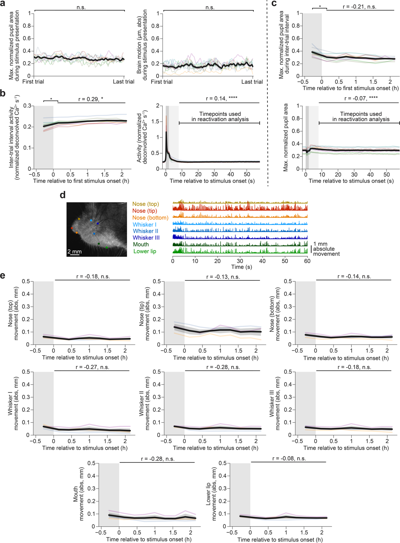
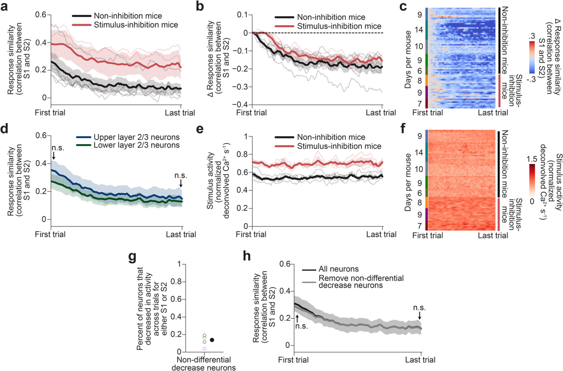
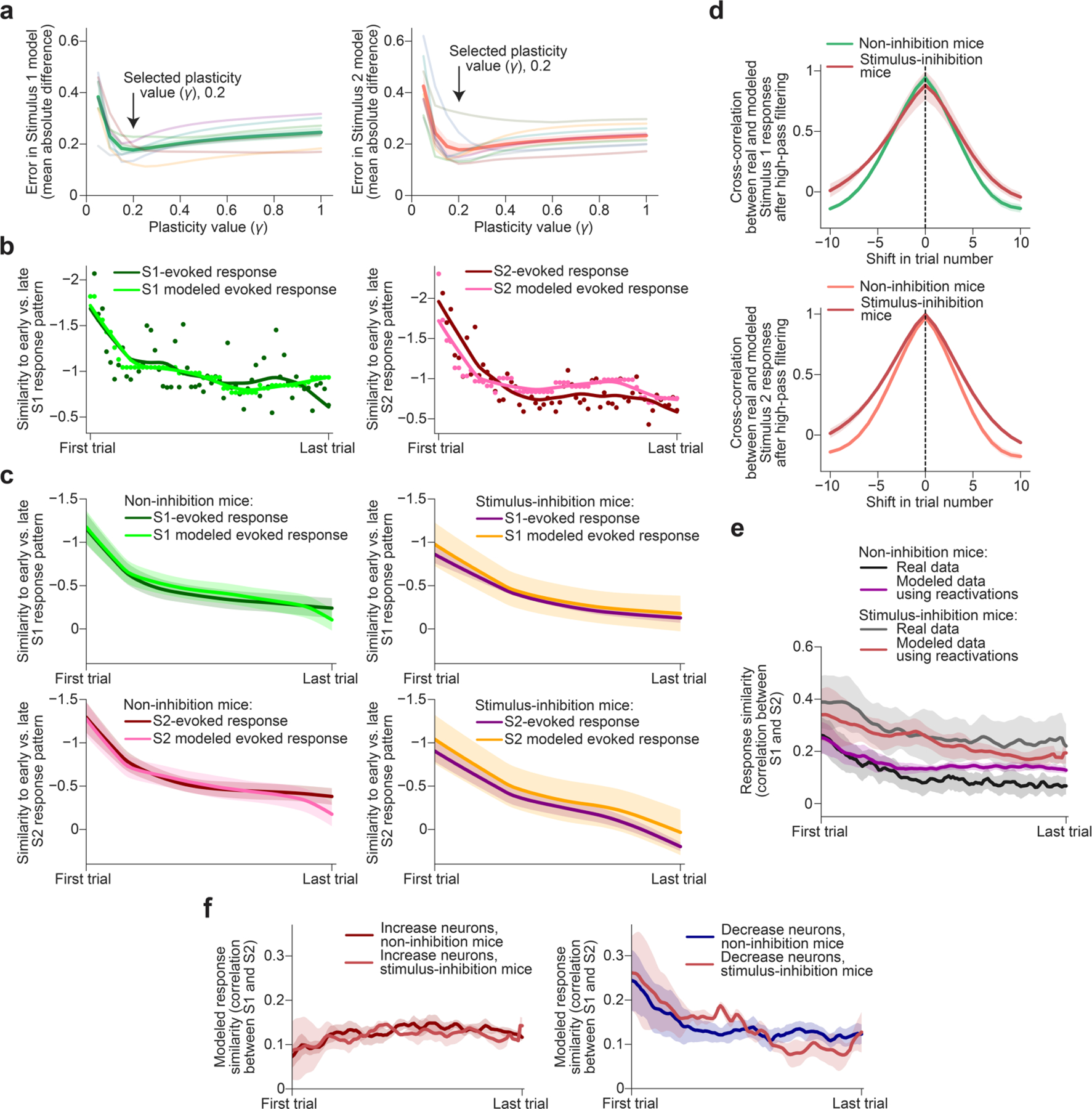
Many theories of offline memory consolidation posit that the pattern of neurons activated during a salient sensory experience will be faithfully reactivated, thereby stabilizing the pattern^1,2. However, sensory-evoked patterns are not stable but, instead, drift across repeated experiences^3-6. Here, to investigate the relationship between reactivations and the drift of sensory representations, we imaged the calcium activity of thousands of excitatory neurons in the mouse lateral visual cortex. During the minute after a visual stimulus, we observed transient, stimulus-specific reactivations, often coupled with hippocampal sharp-wave ripples. Stimulus-specific reactivations were abolished by local cortical silencing during the preceding stimulus. Reactivations early in a session systematically differed from the pattern evoked by the previous stimulus-they were more similar to future stimulus response patterns, thereby predicting both within-day and across-day representational drift. In particular, neurons that participated proportionally more or less in early stimulus reactivations than in stimulus response patterns gradually increased or decreased their future stimulus responses, respectively. Indeed, we could accurately predict future changes in stimulus responses and the separation of responses to distinct stimuli using only the rate and content of reactivations. Thus, reactivations may contribute to a gradual drift and separation in sensory cortical response patterns, thereby enhancing sensory discrimination⁷.

Extended Data Fig. 1 |. Classifying stimulus-specific reactivations.

a, Trial-averaged, deconvolved peri-stimulus Ca²⁺ activity of example neurons driven by S1, S2, or both (“S1 and S2 neurons”). S1- and S2-driven neurons exhibited highly selective responses to their preferred stimulus. b, Quantification of neuron count for: all neurons, S1 and S2 neurons, S1 only neurons, and S2 only neurons (average across all trials, and separately for early and for late trials, n = 8 mice). c, Distribution of selectivity index values (see Methods) of stimulus driven neurons (n = 8 mice). d, Brief summary of method for classifying reactivations (for additional details, see main text and Methods). Left (Step 1): the classifier should identify transient synchronous reactivations that we assume should last at least several hundred milliseconds^,,,,, and thus we estimate population activity patterns using the rolling maximum activity of each cell across ~380 ms. We then remove slow changes in ongoing Ca²⁺ activity by using 3 difference-of-Gaussian filters to high-pass filter activity changes at time scales of 1.5, 6, and 25 s. Middle (Step 2): we define S1 or S2 stimulus reactivations during the inter-trial interval (in which the mouse passively views a mean-luminance blank screen) as epochs of synchronous activity lasting hundreds of milliseconds across neurons driven by stimulus S1 or S2, respectively. To focus on synchronous events, we use a binary prior such that we only classify reactivation pattern content during epochs in which the ongoing activity trace averaged across the top stimulus-driven neurons exceeds 5 standard deviations above the mean. Right (Step 3): we then apply multinomial logistic regression to epochs specified by this temporal prior. We train the classifier on time points that occur during all S1 trials, all S2 trials, and all time points during inter-trial intervals and during the baseline period that do not exhibit synchronous activity of stimulus-driven neurons (temporal prior = 0). We then apply the classifier to all time points with synchronous activity of stimulus-driven neurons during inter-trial intervals and during the baseline period prior to any stimulus presentations (temporal prior = 1). This results in matching probability estimates that the pattern at each time point matches the S1-evoked response pattern, the S2-evoked response pattern (i.e. S1 or S2 reactivation probabilities), or ‘other’ patterns, with the sum of these three probabilities equalling 1 for each time point. e, Reactivation duration during the baseline period before any stimulus presentations vs. during the inter-trial intervals between stimulus presentations (n = 8 mice, two-tailed paired t-test, P = 0.025). f, Left: distribution of reactivation probabilities of the classifier trained using the actual data and trained using data after shuffling using one of two different methods. The first shuffle method defines the temporal prior using an equal number of randomly selected neurons instead of only stimulus-driven neurons, and the second method randomly shuffles the identity of stimulus-driven neurons (n = 8 mice; one-way ANOVA, Holm-Bonferroni corrected, all data points below the significance line indicate classifier probabilities that differ significantly from both shuffled versions, P < .05). Right: fold change in density of each reactivation probability using the actual data as compared to each shuffle (n = 8 mice). We defined reactivation events as those with a peak probability greater than 0.75, as they were greater than three times more common than reactivations detected in shuffled data. g, Reactivation rate during times of synchronous stimulus activity during the ITI vs. all other ITI times with non-synchronous stimulus activity (n = 8 mice, two-tailed paired t-test, P = 3.6 × 10⁻⁷). Classifier probability during the ITI was low outside of moments of synchronous activation of stimulus-driven neurons. In this case, classification of reactivations was performed without removing slow changes in ongoing Ca²⁺ activity using the 3 difference-of-Gaussian filters to preserve all activity during the ITI. h, We confirmed the similarity of stimulus reactivations to stimulus-evoked response patterns by grouping neurons based on their mean response magnitude during stimulus presentations. As expected, the neurons most strongly driven by S1 or S2 were selectively active during S1 or S2 reactivations, respectively. Left: mean S1-evoked activity (green) or S2-evoked activity (red) for the top 5% and bottom 95% of S1- or S2-driven neurons and for other neurons lacking stimulus-evoked Ca²⁺ activity (n = 8 mice, two-tailed paired t-test, Holm-Bonferroni corrected, from left to right: P = 0.0012, P = 1.9 × 10⁻⁴, P = 0.0013, P = 0.0012, P = 0.42). Middle: same as left but for mean Ca²⁺ activity during reactivation events (n = 8 mice, two-tailed paired t-test, Holm-Bonferroni corrected, from left to right: P = 0.0017, P = 6.0 × 10⁻⁴, P = 0.50, P = 0.86, P = 0.55). Right: baseline Ca²⁺ activity (in the 0.5 h prior to any stimulus presentations) for the top 5% and bottom 95% of S1- or S2-driven neurons and for other neurons lacking stimulus-evoked Ca²⁺ activity (n = 8 mice). i, Fraction of neurons that remained in the top 5% of driven neurons during both early trials and late trials (n = 8 mice). Data are mean ± SEM. n.s.: not significant; * P < .05; ** P < .01; *** P < .001; **** P < .0001.

Extended Data Fig. 2 |. Characterizing stimulus reactivations.

a, Mean hippocampal ripple-band power surrounding the onset of classified reactivations (derived from the cortical imaging data) across each session for all mice (n = 14 sessions from 5 mice that differed from the mice used for any other analyses). SD: standard deviations above the mean. b, Brain motion plotted surrounding the onset of classified reactivations (n = 8 mice, two-tailed paired t-test, P = 0.19). c, Phase correlation to the reference frame, plotted surrounding the onset of classified reactivations (n = 8 mice, two-tailed paired t-test, P = 0.011). The phase correlation measures how well each individual frame correlates with the reference frame used for motion correction. d, Peak-normalized pupil movement (absolute change in movement) plotted surrounding the onset of classified reactivation events (n = 8 mice, two-tailed paired t-test, P = 0.47). e, Comparison of mean stimulus-evoked activity (left) or stimulus reactivation activity (right) between neurons located in upper layer 2/3 (~ 156 μm from the brain surface) vs. lower layer 2/3 (~ 266 μm from the brain surface) of lateral visual cortex (n = 8 mice, two-tailed unpaired t-test, stimulus: P = 0.89, reactivation: P = 0.13). f, Change in mean location (centroid, estimated using each stimulus-driven neuron’s activity during reactivations) of stimulus reactivations across the session along the anterior-posterior (left) and lateral-medial axes (right, n = 8 mice, two-tailed paired t-test, Holm-Bonferroni corrected, left: S1: P = 0.035, S2: P = 0.035, right: S1: P = 0.060, S2: P = 0.065). g, Raster plot of ongoing deconvolved Ca²⁺ activity of the top stimulus-driven neurons during and following an example S1 stimulus presentation (green square) and an example S2 stimulus presentation (red square), using all neurons or using a random 10% of neurons (see lower raster). Classification of stimulus reactivations using a random 10% of neurons results in several false positive (blue arrows) and false negative (magenta arrow) classification errors when compared to using all neurons. Inset at right: expanded view of data from green rectangle, illustrating a false-positive classification using a random 10% of neurons. h, Percent of false negative (left) or false positive (right) classifications of reactivations relative to reactivations classified using all neurons, plotted as a function of the percent of randomly selected neurons used in the classifier (n = 8 mice, permutation test, Holm-Bonferroni corrected, P < .05 for all tests). i, Same as h but selecting neurons randomly from the same subregion of the field of view such that they are all close in distance (see Methods, n = 8 mice, permutation test, Holm-Bonferroni corrected, P < .05 for all tests). Data are mean ± SEM. n.s.: not significant; * P < .05.

Extended Data Fig. 3 |. Reactivation rate and bias effects are consistent across sessions and correlate with stimulus novelty and pupil-indexed arousal.

a, Left: reactivation rates (sum of probabilities of S1 or S2 reactivations) across each session, including the 0.5-hour baseline period prior to any stimulus presentations for all daily sessions (n = 5 mice, 48 sessions total). Right: reactivation rate during the inter-trial interval (n = 5 mice, 48 sessions total) for all daily sessions. b, Left: bias index of reactivation content (positive values indicate bias towards the most recent stimulus, n = 5 mice, 48 sessions total) for all daily sessions. Right: bias throughout the inter-trial interval (n = 5 mice, 48 sessions total) for all daily sessions. c, Reactivation content bias during stimulus presentations across the session using all neurons vs. a random 10% of neurons (n = 8 mice, permutation test between mean of traces, P = 0.0016). d, Stimulus reactivation rates when the stimulus on the preceding trial was different vs. when it was the same as on the current trial (n = 8 mice, one-tailed t-test vs. 0, P = 9.8 × 10⁻⁴). e, Correlation between pupil area during stimulus presentation and stimulus reactivation rate during the subsequent ITI (n = 8 mice, one-tailed t-test vs. 0, P = 0.026). f, Correlation between stimulus activity during stimulus presentation and stimulus reactivation rate during the subsequent ITI (n = 8 mice, one-tailed t-test vs. 0, P = 0.033). Data are mean ± SEM. n.s.: not significant; * P < .05; ** P < .01; *** P < .001.

Extended Data Fig. 4 |. Physical correlates of arousal remain constant throughout the session.

a, Left: peak-normalized pupil area during stimulus presentations across trials (n = 8 mice, two-tailed paired t-test, P = 0.056). Right: brain motion during stimulus presentations across trials (n = 8 mice, two-tailed paired t-test, P = 0.48). Coloured lines: individual mice. Black line: mean across mice. b, Left: Ca²⁺ activity during the baseline period before any stimulus presentation (dark shaded region) and during inter-trial intervals between stimulus presentations (n = 8 mice, two-tailed paired t-test, P = 0.016, two-tailed linear least-squares regression, P = 0.018, Holm-Bonferroni corrected). Right: Ca²⁺ activity during stimulus presentation and throughout the inter-trial interval (n = 8 mice, two-tailed linear least-squares regression, P = 1.2 × 10⁻¹⁹). Dark shaded region: stimulus presentation. Light shaded region: excluded portion of inter-trial interval. Coloured lines: individual mice. Black line: mean across mice. c, Top: peak-normalized pupil area during the baseline period before any stimulus presentation and during inter-trial intervals between stimulus presentations (n = 8 mice, two-tailed paired t-test, P = 0.019, two-tailed linear least-squares regression, P = 0.092, Holm-Bonferroni corrected). Bottom: peak-normalized pupil area during stimulus presentation and throughout the inter-trial interval (n = 8 mice, two-tailed linear least-squares regression, P = 1.7 × 10⁻⁶). Dark shaded region: stimulus presentation. Light shaded region: excluded portion of inter-trial interval. Coloured lines: individual mice. Black line: mean across mice. d, Left: example image from a recording of the mouse’s face during imaging. Each coloured dot denotes a keypoint on the face that was tracked across each session. Right: example traces of 8 tracked keypoints on the nose, whiskers, and mouth (nose top, nose tip, nose bottom, whiskers I-III, mouth, and lower lip). Traces are in units of absolute movement. e, Absolute movement of 8 tracked keypoints (nose top, nose tip, nose bottom, whiskers I-III, mouth, and lower lip) during the baseline period before any stimulus presentation and during 2.5 h of stimulus presentations (n = 3 mice, two-tailed linear least-squares regression, nose top: P = 0.39, nose tip: P = 0.54, nose bottom: P = 0.51, whisker I: P = 0.21, whisker II: P = 0.18, whisker III: P = 0.40, mouth: P = 0.19, lower lip: P = 0.70). Data are mean ± SEM. n.s.: not significant; * P < .05; **** P < .0001.

Extended Data Fig. 5 |. Characterizing the effects of peri-stimulus inhibition.

a, Coronal sections of visual cortex displaying virally-mediated expression of Cre-dependent jGCaMP7s in glutamatergic neurons (green, in Emx1-Cre mice) and Chrimson in parvalbumin interneurons (red, S5E2 enhancer) in 3 mice. Local injections ensured targeted expression of Chrimson throughout lateral visual cortical areas in all 3 mice. b, Left: stimulus-evoked Ca²⁺ activity during control vs. stimulus-inhibition trials (n = 3 mice, two-tailed paired t-test, P = 0.0056). Right: percent reduction in Ca²⁺ activity on stimulus-inhibition trials compared to control trials (n = 3 mice, one-sample t-test vs. 0, P = 0.0022). For stimulus-inhibition trials, we pulsed 10 mW of red light for 4 ms at 16 Hz from 1 s before stimulus onset to 1 s after stimulus offset. c, Peak-normalized pupil area during stimulus presentation and during the inter-trial interval for control vs. stimulus-inhibition trials (n = 3 mice, two-tailed paired t-test between mean of traces during the stimulus period plus the period immediately following the stimulus, P = 0.75, or during the specified inter-trial interval, P = 0.76, Holm-Bonferroni corrected). Red horizontal bar at top indicates timing of optogenetic silencing. Noise bars indicate time of visual stimulus. Grey shaded area indicates post-stimulus period excluded from reactivation analyses. d, Ca²⁺ activity during stimulus presentation and during the inter-trial interval for control vs. stimulus-inhibition trials (n = 3 mice, two-tailed paired t-test between mean of traces during the specified inter-trial interval, P = 0.19). Red horizontal bar at top indicates timing of optogenetic silencing. Noise bars indicate time of visual stimulus. Grey shaded area indicates post-stimulus period excluded from reactivation analyses. e, Reactivation rate during the inter-trial interval for all stimulus-inhibition trials that were proceeded by a control trial (n = 3 mice, two-tailed linear least-squares regression, Holm-Bonferroni corrected, control trials: P = 0.016, stimulus-inhibition trials: P = 0.38). f, Pupil size-matched reactivation rate during the baseline period before stimulus presentation and during the ITI following stimulus-inhibition trials (n = 3 mice, two-tailed paired t-test, P = 0.018). Times were selected such that the mean pupil size between the two conditions was identical (see Methods). g, Bias index of reactivation content during the inter-trial interval for all stimulus-inhibition trials that were proceeded by a control trial (n = 3 mice, two-tailed linear least-squares regression, Holm-Bonferroni corrected, control trials: P = 0.40, stimulus-inhibition trials: P = 0.66). Here, the bias index is calculated throughout as the bias in reactivation content towards the stimulus presented on the control trial (black vertical line). h, Mean reactivation rate for non-inhibition mice (n = 5 mice) across all trials and for stimulus-inhibition mice (n = 3 mice) across all trials or control (no-inhibition) trials (two-tailed unpaired t-test, Holm-Bonferroni corrected, non-inhibition mice all trials vs. stimulus-inhibition mice all trials: P = 0.11, non-inhibition mice all trials vs. stimulus-inhibition mice control trials: P = 0.019). Data are mean ± SEM. n.s.: not significant; * P < .05; ** P < .01.

Extended Data Fig. 6 |. Compared to non-inhibition mice, stimulus-inhibition mice exhibit similar stimulus response orthogonalization but higher response magnitudes during control trials.

a, Response similarity shown separately for non-inhibition mice (n = 5 mice) and stimulus-inhibition mice (n = 3 mice; using no-inhibition control trials only). b, Change in response similarity (same as a but after subtracting the mean response similarity in first 3 trials) shown separately for non-inhibition mice (n = 5 mice) and stimulus-inhibition mice (n = 3 mice). c, Heatmap of change in response similarity shown separately for non-inhibition mice (n = 5 mice) and stimulus-inhibition mice (n = 3 mice) for all sessions. d, Response similarity using neurons located in upper layer 2/3 or lower layer 2/3 (n = 8 mice, two-tailed unpaired t-test between the mean of the first or last 3 datapoints of the two traces, Holm-Bonferroni corrected, first: P = 0.74, last: P = 0.85). e, Mean stimulus-evoked activity per trial (across all S1 and S2 trials) averaged across all stimulus-driven neurons shown separately for non-inhibition mice (n = 5 mice) and stimulus-inhibition mice (n = 3 mice; using control trials only). f, Heatmap of mean stimulus-evoked activity shown separately for non-inhibition mice (n = 5 mice) and stimulus-inhibition mice (n = 3 mice) for all sessions. g, Percent of decrease neurons that showed a similar decrease in response to both S1 and S2 (defined as a similar drop in Ca²⁺ events/second and/or a similar proportional drop in response magnitude to S1 and S2, n = 8 mice). h, Response similarity when using all neurons or when omitting non-differential decrease neurons (n = 8 mice, permutation test between the mean of the first or last 3 datapoints of the two traces, Holm-Bonferroni corrected, first: P = 0.73, last: P = 0.79). Data are mean ± SEM. n.s.: not significant.

Extended Data Fig. 7 |. Tracking the same neurons across days.

a, Left: example zoom-in of the same subregion of a field of view across six days of imaging. Green, orange, purple, and red boxes highlight the same neurons tracked across all six days. Right: example neurons and masks tracked across six days of imaging, colour-matched to the neurons outlined in the left panel. b, The number of neurons tracked across all six days of imaging (n = 5 non-inhibition mice). c, Change in response similarity from the end of the previous day to the start of the next day across six days of imaging (n = 5 non-inhibition mice, two-tailed paired t-test, P = 0.42). Positive values indicate an increase in response similarity, reflecting a partial relapse in response similarity. Data are mean ± SEM. n.s.: not significant.

Extended Data Fig. 8 |. Characterization of no-change, increase, and decrease neurons.

a, Mean stimulus-evoked activity across trials shown separately for non-inhibition mice (n = 5 mice) and stimulus-inhibition mice (n = 3 mice, control trials only) for no-change (left), increase (middle), or decrease (right) neuron groups. b, Numbers of neurons that are characterized as no-change, increase, or decrease neurons (n = 8 mice). c, Baseline activity before any stimulus presentation for no-change, increase, and decrease neurons (n = 8 mice, one-way ANOVA, Tukey HSD corrected, P > .05 for all tests). d, Percent of all neurons in visual region LI, POR, P, or LM that were defined as no-change, increase, or decrease neurons (n = 8 mice, one-way ANOVA, Tukey HSD corrected, P > .05 for all tests). e, Percent of all neurons in upper layer 2/3 or in lower layer 2/3 that were characterized as no-change, increase, or decrease neurons (n = 8 mice, two-tailed unpaired t-test, Holm-Bonferroni corrected, P > .05 for all tests). f, Within-group noise correlation (see Methods) of no-change, increase, or decrease neurons (n = 8 mice, one-way ANOVA, Tukey HSD corrected, P > .05 for all tests). g, Response similarity (running correlation between response patterns during neighbouring S1 and S2 trials), plotted in the same manner as the mean trace in Fig. 3g for increase neurons (left) and decrease neurons (right), but shown separately for non-inhibition mice (n = 5 mice) and stimulus-inhibition mice (n = 3 mice). h, Fraction of neurons that increase or decrease their stimulus selectivity (selectivity index: (S1_response – S2_response) / (S1_response + S2_response); see Methods) from early to late trials for no-change, increase, or decrease neurons, shown separately for non-inhibition mice (n = 5 mice) and stimulus-inhibition mice (n = 3 mice). i, Cross-correlation between high-pass filtered (see Methods) response similarity and reactivation probability traces shown separately for non-inhibition mice (n = 5 mice) and stimulus-inhibition mice (n = 3 mice). Data are mean ± SEM. n.s.: not significant.

Extended Data Fig. 9 |. Stimulus reactivations consistently predict future stimulus responses.

a, For each trial, we projected single-trial response patterns (during S1 or S2) and stimulus-specific reactivations during the inter-trial interval (S1R or S2R) onto the axis between early and late stimulus-evoked response patterns within a session (see Fig. 4a, b for additional graphical details). Here, data from a typical example session is shown. b, Same as a but for the mean across all sessions and mice shown separately for non-inhibition mice (n = 5 mice) and stimulus-inhibition mice (n = 3 mice). c, Same as Fig. 4b but shown separately for each of the first six days of imaging per mouse, using all neurons that were tracked across the six days (n = 5 non-inhibition mice). The change in overall y-axis offset per day is not meaningful in this case since each projection uses a different projection axis estimated on each day ‘i’, i = 1–6. d, Same as Fig. 4b but using only neurons from upper layer 2/3 or from lower layer 2/3 (n = 8 mice, permutation test between the mean of the first or last 3 datapoints of the upper layer vs. lower layer traces, Holm-Bonferroni corrected, P > .05 for all tests). e, Same as Fig. 4b but after removing non-differential decrease neurons (see Extended Data Fig. 6g, n = 8 mice, permutation test between the mean of the first or last 3 datapoints of the traces generated using data from all neurons vs. from all neurons after removing non-differential decrease neurons, Holm-Bonferroni corrected, P > .05 for all tests). f, Ratio of mean activity across trials early in each session in increase (top) or decrease (bottom) neurons relative to no-change neurons during S1 presentations vs. S1R reactivation events, and during S2 presentations vs. S2R reactivation events, shown separately for non-inhibition mice (n = 5 mice) and stimulus-inhibition mice (n = 3 mice). g, Stimulus-evoked activity vs. reactivation activity, averaged across all stimulus-driven neurons (n = 8 mice). h, Difference between a neuron’s 1.3x-scaled peri-reactivation activity and its peri-stimulus activity early in each session, averaged across neurons in each group, and shown separately for non-inhibition mice (n = 5 mice) and stimulus-inhibition mice (n = 3 mice). i, Difference between a neuron’s 1.3x-scaled peri-reactivation activity and its peri-stimulus activity early in each session for S1 and S2 trials for neurons that change their stimulus preference (from early to late trials), either from being driven only by S1 to being driven only by S2 (top) or from being driven only by S2 to being driven only by S1 (bottom, n = 8 mice, two-tailed paired t-test, top: P = 3.7 × 10⁻⁴, bottom: P = 0.0034). Data are mean ± SEM. n.s.: not significant; ** P < .01; *** P < .001.

Extended Data Fig. 10 |. Modelling future stimulus responses using only stimulus reactivations.

a, We parametrically varied the plasticity variable γ and measured the error in the modelled stimulus-evoked response patterns vs. actual stimulus-evoked response patterns (mean of the absolute difference between actual and modelled data). The value of 0.2 had the least mean error for both S1 and S2 (n = 8 mice). We used this same value for modelling all sessions and mice. This value is likely an overestimate as we do not consider plasticity that occurs during the stimulus response period. b, Comparison of projection of the actual stimulus-evoked response patterns (dark green/red dots and smoothed trace) with the modelled patterns (light green/pink dots and smoothed trace), projected onto V_s for a single session. c, Comparison of projection of the actual stimulus-evoked response patterns with the modelled patterns, projected onto V_s across all days and mice, shown separately for non-inhibition mice (n = 5 mice) and stimulus-inhibition mice (n = 3 mice). d, Cross-correlation between high-pass filtered actual and modelled projections of stimulus-evoked response patterns shown separately for non-inhibition mice (n = 5 mice) and stimulus-inhibition mice (n = 3 mice, see Methods). e, Response similarity as measured by the correlation between the mean response patterns during nearby S1 and S2 trials, plotted for actual and modelled stimulus responses, shown separately for non-inhibition mice (n = 5 mice) and stimulus-inhibition mice (n = 3 mice). f, Response similarity using modelled data, for increase or decrease neuron groups, shown separately for non-inhibition mice (n = 5 mice) and stimulus-inhibition mice (n = 3 mice). As in Fig. 3g, only decrease neurons show orthogonalization across trials, and this was evident in both sets of mice.

Fig. 1 |. Distributed stimulus reactivations in the lateral visual cortex during quiet waking.

a, Two-photon imaging in awake head-fixed mice during repeated, passive presentation of S1 or S2. The stimuli (2 s duration, 58 s ITI) were presented in a random order for 2.5 h. b, Cre-dependent jGCaMP7s expression in glutamatergic neurons through local injections across the visual cortex in Emx1-cre mice (top). Bottom, epifluorescence retinotopic mapping identified visual cortical areas: primary visual cortex (V1), lateromedial (LM), postrhinal (POR), laterointermediate (LI) and posterior (P). Simultaneous wide-field two-photon Ca²⁺ imaging of approximately 6,900 neurons across 3 depths within layer 2/3 (white rectangle). Bottom right, example magnified subregion. Scale bars, 0.5 mm (left) and 0.2 mm (right). A, anterior; P, posterior; L, lateral; M, medial. c, Trial-averaged, deconvolved peri-stimulus Ca²⁺ activity from an example session sorted by stimulus preference. d, Raster plot of ongoing deconvolved Ca²⁺ activity of the top S1-driven and S2-driven neurons for three example trials. We used multinomial logistic regression (Methods and Extended Data Fig. 1d) to decode whether synchronous patterns during the ITI resembled the S1-evoked pattern (S1 reactivation probability; green) or the S2-evoked pattern (S2 reactivation probability; red). e, The mean pupil area (normalized to the maximum across the session (top) and the relative change (bottom)) surrounding the onset of reactivations. n = 8 mice. Statistical analysis was performed using two-tailed paired t-tests; P = 0.0039 (top), P = 0.0019 (bottom). f, Same analysis as in e but for ripple-band power of the local field potential measured in the dorsal hippocampal CA1. n = 5 mice. Statistical analysis was performed using a two-tailed paired t-test; P = 0.011. g, Example stimulus-evoked response of stimulus-driven neurons across the lateral visual cortex (left). Right, mean stimulus-evoked activity of LI, POR, P and LM neurons. n = 8 mice. Statistical analysis was performed using one-way analysis of variance (ANOVA) with correction using Tukey’s honest significant difference (HSD) test; P > 0.05 for all tests. h, Same analysis as in g but for stimulus reactivation activity (P > 0.05 for all tests). For g and h, scale bars, 0.25 mm. Data in e–h are mean ± s.e.m. NS, not significant; *P < 0.05; **P < 0.01.

Fig. 2 |. Cortical responses to stimuli drive subsequent reactivations.

a, Example single-session raster plot of S1 and S2 reactivations (green and red dots) after the presentation of S1 or S2. b, Left, the reactivation rate across the session, including the 0.5 h baseline period before any stimulus presentations (dark shaded region). n = 5 mice. Statistical analysis was performed using a paired t-test (P = 7.7 × 10⁻⁴) and linear least-squares regression (P = 2.7 × 10⁻⁵) with Holm–Bonferroni correction. Right, the reactivation rate during the ITI. n = 5 mice. Statistical analysis was performed using linear least-squares regression; P = 0.0067. c, Left, the bias index of reactivation content (positive values indicate bias towards the most recent stimulus; Methods). n = 5 mice. Statistical analysis was performed using linear least-squares regression; P = 0.025. Right, bias throughout the ITI. n = 5 mice. Statistical analysis was performed using linear least-squares regression; P = 3.9 × 10⁻⁴. d, Schematic and mean in vivo image of selective viral expression of jGCaMP7s and Chrimson-tdTomato in lateral visual cortical glutamatergic neurons (Emx1-cre) and parvalbumin interneurons (due to S5E2 enhancer), respectively. Scale bar, 0.1 mm. e, The mean stimulus-evoked activity of driven neurons across trials from one example session. On 50% of trials, stimulus-evoked activity was suppressed from 1 s before to 1 s after stimulus presentation (light green and pink bars, stimulus-inhibition trials) using optogenetics (Methods). f, The same analysis of reactivation rate as described in b but for control versus inhibition trials. n = 3 mice. Statistical analysis was performed using paired t-tests between the mean of traces; P = 0.0025 (left), P = 0.0039 (right). g, The bias index as described in c but for control versus inhibition trials. n = 3 mice. Statistical analysis was performed using paired t-tests between the mean of traces; P = 0.029 (left), P = 0.010 (right). Data in b,c,f,g are mean ± s.e.m. *P < 0.05; **P < 0.01; ***P < 0.001; ****P < 0.0001. Light shaded regions show the excluded portion of the ITI. White-noise bars in b,c,f,g indicate the stimulus presentation. All of the statistical tests were two-tailed.

Fig. 3 |. Progressive separation of stimulus response patterns correlates with reactivation rate.

a, Example early and late S1 trials. b, Response similarity (Methods). n = 8 mice. Statistical analysis was performed using linear least-squares regression; P = 5.2 × 10⁻²². Data are from 5 mice with approximately 120 trials per session and 3 mice with approximately 60 control (no inhibition) trials per session. c, Stimulus-evoked activity. n = 8 mice. Statistical analysis was performed using a paired t-test (P = 0.095) and linear least-squares regression (P = 0.090). d, Response similarity as described in b but plotted across days (n = 5 mice) using the same tracked neurons. e, Response similarity at start or end of each day in d. n = 5 mice. Statistical analysis was performed using paired t-tests; P = 0.0026 (left), P = 0.030 (right). f, Stimulus-evoked activity as described in c but for no-change, increase or decrease neurons. n = 8 mice. Statistical analysis was performed using unpaired t-tests with Holm–Bonferroni correction; P = 4.0 × 10⁻¹² (red), P = 4.0 × 10⁻¹¹ (blue). g, Response similarity as described in b but for increase or decrease neurons. n = 8 mice. Statistical analysis was performed using linear least-squares regression with Holm–Bonferroni correction; P = 3.6 × 10⁻⁴ (red), P = 1.4 × 10⁻⁶⁰ (blue). h, The fraction of neurons that increase or decrease their stimulus selectivity from early to late trials for each group. n = 8 mice. Statistical analysis was performed using paired t-tests with Holm–Bonferroni correction; P > 0.05 (no-change neurons and increase neurons), P = 0.025 (decrease neurons). i, Example response similarity and reactivation rate traces. j, Correlation between the two variables for unfiltered traces (left) and after high-pass filtering (right). n = 8 mice. Statistical analysis was performed using t-tests versus 0; P = 1.3 × 10⁻⁴ (left), P = 7.9 × 10⁻⁹ (right). k, Cross-correlation between high-pass-filtered response similarity and reactivation probability traces. n = 8 mice. Data in b–h,j,k are mean ± s.e.m. All statistical tests were two-tailed. NS, not significant; *P < 0.05; **P < 0.01; ***P < 0.001; ****P < 0.0001.

Fig. 4 |. Reactivations predict representational drift.

a, Schematic of drifting stimulus response patterns along V_s. V_s denotes the vector along the axis from early to late response patterns. b, Projection of S1-evoked response patterns and reactivations onto V_s (left). Right, the same but for S2. n = 8 mice. Statistical analysis was performed using paired t-tests; P = 1.3 × 10⁻⁴ (left), P = 1.5 × 10⁻⁴ (right). c, Projection of S1- and S2-evoked response patterns and reactivations onto V_s as described in b but across days using tracked neurons and projected onto the day 1 axis. n = 5 mice. Statistical analysis was performed using paired t-tests; P = 5.0 × 10⁻⁴ (left), P = 3.7 × 10⁻⁴ (right). d, S1- and S2-evoked response patterns and reactivations as in c but projected onto the day 1 to 6 axis. n = 5 mice. Statistical analysis was performed using paired t-tests; P = 9.0 × 10⁻⁴ (left), P = 3.8 × 10⁻⁴ (right). e, Left, early-trial activity of increase neurons relative to no-change neurons during stimulus presentation (S1 or S2) versus reactivations (S1R or S2R). Right, the same but for decrease neurons. n = 8 mice. Statistical analysis was performed using paired t-tests with Holm–Bonferroni correction; from left to right, P = 1.4 × 10⁻⁸, P = 3.0 × 10⁻⁸, P = 1.6 × 10⁻⁵, P = 1.0 × 10⁻⁷. f, Early-trial 1.3×-scaled reactivation activity minus stimulus activity. n = 8 mice. Statistical analysis was performed using one-way ANOVA with correction using Tukey’s HSD test; left: P = 2.6 × 10⁻⁸ (increase versus decrease), P = 0.0068 (increase versus no-change), P = 3.1 × 10⁻⁵ (no-change versus decrease); right: P = 3.2 × 10⁻⁷ (increase versus decrease), P = 0.021 (increase versus no-change), P = 2.0 × 10⁻⁴ (no-change versus decrease). g, Model using reactivations to predict future stimulus responses. h, Comparison of actual versus modelled projection. n = 8 mice. Insets: cross-correlation between high-pass-filtered actual and modelled projections. i, The response similarity for actual versus modelled data. n = 8 mice. Statistical analysis was performed using paired t-tests with Holm–Bonferroni correction; P = 0.13 (first), P = 0.18 (last). j, Response similarity as in Fig. 3g, but for modelled data. n = 8 mice. Statistical analysis was performed using linear least-squares regression with Holm–Bonferroni correction; P = 1.8 × 10⁻¹³ (red), P = 1.7 × 10⁻⁴³ (blue). k, Summary. S1- and S2-evoked response patterns are pulled towards their respective reactivation pattern across trials. Data in b–f,h–j are mean ± s.e.m. All statistical tests were two-tailed. NS, not significant; *P < 0.05; **P < 0.01; ***P < 0.001; ****P < 0.0001.

References

1. Foster DJ Replay comes of age. Annu. Rev. Neurosci 40, 581–602 (2017). - PubMed
1. Tambini A & Davachi L Awake reactivation of prior experiences consolidates memories and biases cognition. Trends Cogn. Sci 23, 876–890 (2019). - PMC - PubMed
1. Failor SW, Carandini M & Harris KD Visuomotor association orthogonalizes visual cortical population codes. Preprint at bioRxiv 10.1101/2021.05.23.445338 (2022). - DOI
1. Schoonover CE et al. Representational drift in primary olfactory cortex. Nature 594, 541–546 (2021). - PubMed
1. Marks TD & Goard MJ Stimulus-dependent representational drift in primary visual cortex. Nat. Commun 12, 5169 (2021). - PMC - PubMed
LinkOut - more resources