Large-scale single-neuron speech sound encoding across the depth of human cortex

Abstract

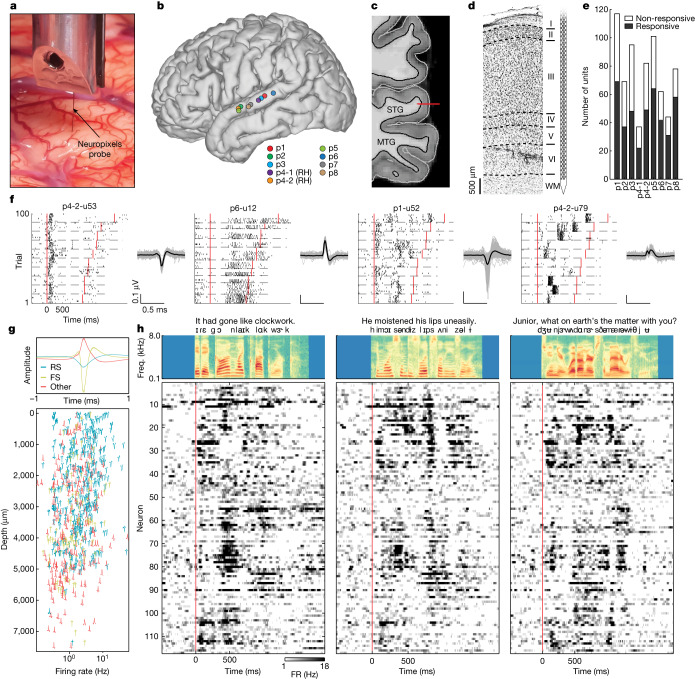
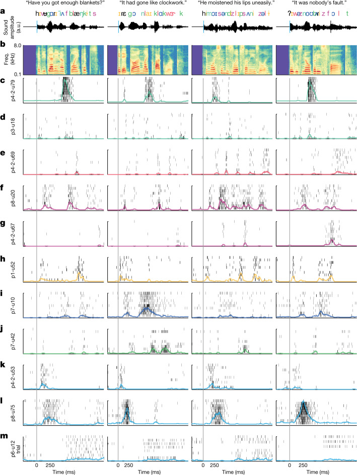
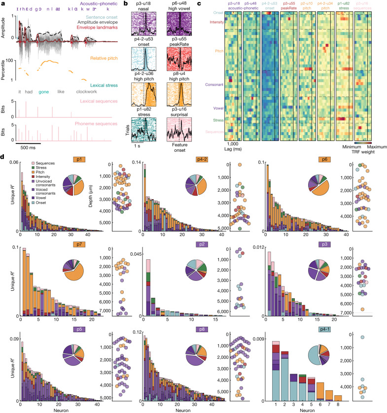
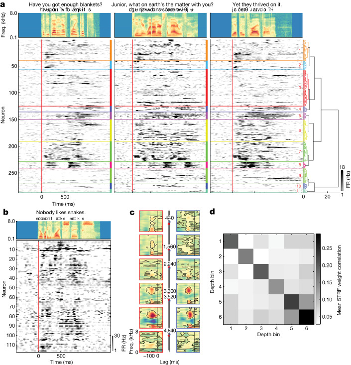
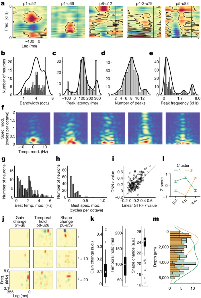
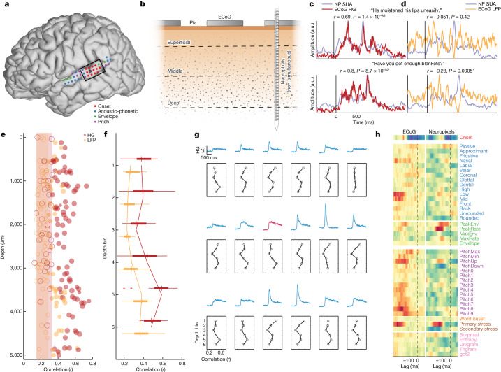
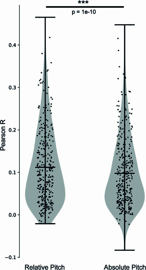
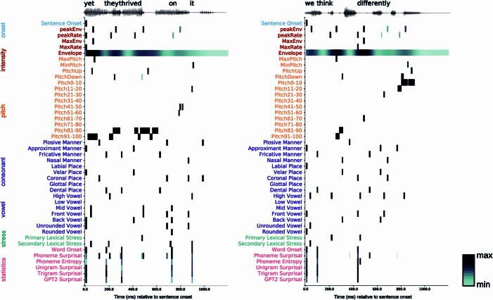
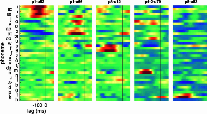
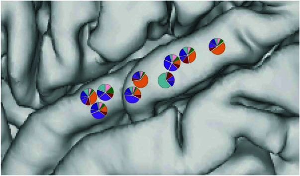
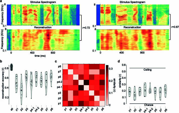
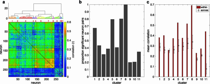
Understanding the neural basis of speech perception requires that we study the human brain both at the scale of the fundamental computational unit of neurons and in their organization across the depth of cortex. Here we used high-density Neuropixels arrays^1-3 to record from 685 neurons across cortical layers at nine sites in a high-level auditory region that is critical for speech, the superior temporal gyrus^4,5, while participants listened to spoken sentences. Single neurons encoded a wide range of speech sound cues, including features of consonants and vowels, relative vocal pitch, onsets, amplitude envelope and sequence statistics. Neurons at each cross-laminar recording exhibited dominant tuning to a primary speech feature while also containing a substantial proportion of neurons that encoded other features contributing to heterogeneous selectivity. Spatially, neurons at similar cortical depths tended to encode similar speech features. Activity across all cortical layers was predictive of high-frequency field potentials (electrocorticography), providing a neuronal origin for macroelectrode recordings from the cortical surface. Together, these results establish single-neuron tuning across the cortical laminae as an important dimension of speech encoding in human superior temporal gyrus.

Fig. 1. Large-scale human single-neuron recording across the cortical depth using Neuropixels probes.

a, Close-up photograph of the Neuropixels probe inserted into the human cortex. b, Recording locations for nine penetrations (right STG sites (RH) plotted on the left hemisphere). c, Magnetic resonance imaging shows the approximate location of the Neuropixels probe spanning the full cortical depth in p1 (MTG, middle temporal gyrus). d, Histology from resected tissue at the insertion site in p1 provides approximate laminar boundaries within STG. e, Number of speech-responsive and non-responsive units. f, Single-trial spike rasters for example neurons showing how neurons respond differently to different sentences. Each neuron shows multiple trials of 10 different sentences (separated by dashed lines). Spike waveforms (mean and 100 randomly selected single spikes) are shown to the right. Red lines indicate sentence onset and offset. g, Three types of spike waveform (upper panel; FS, fast spiking; RS, regular spiking) with distribution across the cortical depth in nine sites (lower panel). h, Thresholded PSTH (50 ms window) for three sentences (averaged across repetitions) from 117 neurons in p1 (sorted by depth) shows patterns of evoked activity across the depth. The upper panels show acoustic spectrograms of each sentence with word and phoneme annotations. freq., frequency; FR, firing rate.

Fig. 2. Single-trial rasters for example neurons show diversity of response types and tuning.

a, Four example sentences with word- and phoneme-level transcriptions time aligned to the audio waveform. Phoneme/feature colours correspond to example units in c–m, which were labelled by hand for visualization purposes. b, Acoustic spectrogram of speech stimuli. Rasters for each neuron and sentence. Rows correspond to the number of repeats for that neuron and sentence. Coloured lines are the smoothed (50 ms window) PSTHs across trials. c,d, Two examples of neurons responding primarily to nasal sounds (for example, /m/, /n/). Note that even similarly tuned neurons can have very different spiking properties (for example, primarily bursting (p4-2-u79) versus sparse firing (p3-u18)). e, Neuron responding primarily to approximant sounds (for example, /l/, /r/, /w/). f,g, Two examples of neurons that are selectively responsive to fricatives (for example, /s/, /z/, /f/). h, Neuron selectively responsive to high/front vowels (for example, /i/, /ɪ/). i, Neuron primarily responsive to low/back vowels (for example, /ɑ/, /ʌ/, /ɔ/). j, Neuron primarily responsive to plosives (for example, /b/, /d/, /g/, /p/, /t/, /k/). k–m, Neurons responsive to sentence onsets. Some units show increased firing at onset (k,l), whereas others show delayed firing (m). a.u., arbitrary unit.

Fig. 3. Encoding of heterogeneous speech features within and across cortical sites.

a, Example sentence annotations with acoustic–phonetic (vowel, consonant), prosodic (relative pitch, intensity, stress, onset) and sequence statistics features. b, Spike rasters for eight neurons aligned to a subset of speech features. The y axis corresponds to all instances of the given feature (for example, all nasal sounds across all sentences). The x axis is aligned to the feature of interest (plus or minus 1 s). The black lines indicate the average response to all feature instances. c, TRF weights from the full encoding model for a set of example neurons, demonstrating encoding of specific speech properties. Only feature class labels are shown (Extended Data Fig. 3 and Supplementary Table 1 show all individual feature labels). d, Unique variance for each class of speech feature on all significant neurons in each cortical site. Bar graphs show a breakdown of unique R² for each neuron, which is derived from a comparison between variance explained by the full model and variance explained by a reduced model with a given feature class removed. Large pie charts show the proportion of explained variance attributed to each feature class across neurons. Small scatterplots (on the right) show the dominant feature for each neuron sorted by depth (the x axes are arbitrary for visualization). Coloured boxes around participant numbers indicate the dominant feature class for the site.

Fig. 4. Neuronal activity is clustered by response type and cortical depth.

a, Evoked responses for three example sentences for neurons with significant TRFs (Fig. 3) sorted by hierarchical clustering (Extended Data Fig. 7). b, An example PSTH from one site for one sentence (averaged over repetitions) shows variable response types at different depths. c, Example STRFs from one site show different tuning across depth and similar tuning for nearby neurons (left versus right). Numbers refer to neuron depth (micrometres). d, Correlation of STRF weights for neurons binned into six groups by depth (bin 1 is most superficial) averaged across all sites.

Fig. 5. Encoding models reveal broad and diverse patterns of spectrotemporal tuning in STG neurons.

a, STRFs for example neurons show distinct patterns of spectrotemporal tuning. b, Across all significant STRFs (permutation test versus shuffled distribution), tuning was broad, with mean bandwidth of approximately four octaves. c, STG neurons showed early-to-mid peak latency responses (approximately 150 ms). d, Most neurons had tuning to multiple spectral peaks. e, Frequency tuning was focused in the range of human voicing (less than 500 Hz). f, Modulation transfer functions for the same example neurons show diverse tuning for spectral and temporal modulations in speech. g, Across all neurons with significant STRFs, temporal modulations were focused at approximately 0.5 Hz and approximately 2.5 Hz. h, Spectral modulations were generally less than 0.5 cycles per octave. i, Comparison between linear STRF and DNN. j, Example dSTRFs for three neurons illustrate three types of nonlinearities: gain change, temporal hold and shape change. Rows are different time steps. k, Distribution of nonlinearities across the population of neurons with significant dSTRFs of each type (n = 189; box plots show the maximum and minimum values (whiskers), median (centre line) and the 25th to 75th percentiles (box limits)). l, Average (plus or minus s.e.m.) Z-scored nonlinearities for dSTRFs categorized using unsupervised hierarchical clustering (Supplementary Fig. 3) (cluster 1 n = 110, cluster 2 n = 79) showing high weight for one or two types of nonlinearities across the population. m, The two clusters have different distributions across cortical depth, with cluster 1 (gain change (g.c.)/temporal hold (t.h.)) being deeper than cluster 2 (shape change (s.c.)). oct., octave; spec. mod., spectral modulation; temp. mod., temporal modulation.

Fig. 6. High-frequency population activity at the cortical surface reflects contributions from single neurons throughout the cortical depth.

a, ECoG electrodes over STG from p1. Colour indicates the top feature in the speech encoding model for each ECoG electrode. The Neuropixels site is highlighted in black, and the black box notes the electrodes shown in g. b, Schematic of surface ECoG (macroelectrodes) and SUA across the cortical depth recorded with Neuropixels (not recorded simultaneously with ECoG). c, Example evoked responses to two sentences with average SUA from Neuropixels (NP) and ECoG high gamma at the same site in STG (Pearson r, two-sided test). d, Example evoked responses to the same two sentences with average SUA and ECoG LFP (Pearson r, two-sided test). e, Correlation between SUA PSTH activity and ECoG high gamma/LFP for each neuron in p1. Open circles and shaded regions indicate non-significance. f, Correlations in d (n = 117) binned into six depth ranges show contributions from all depths, particularly the deepest bins (box plots show the maximum and minimum values (whiskers), median (centre line) and the 25th to 75th percentiles (box limits)). g, Average evoked responses across sentences for ECoG electrodes across STG (top and middle traces; the red trace is the site of the Neuropixels probe). Bottom subplots show binned depth correlations as in f. h, TRF encoding model weights for ECoG (left) and average SUA (weighted by model r; right) show similar patterns. HG, high gamma.

Extended Data Fig. 1. Histology from three additional recording sites.

Each Nissl stain is from fixed tissue that was sectioned to cover the region immediately surrounding the Neuropixels insertion site. Attempts were made to localize the insertion site, but this was very difficult to do with standard anatomic pathology sampling. Therefore, we have provided images from approximately the same area.

Extended Data Fig. 2. Relative versus absolute pitch encoding.

The reconstruction accuracy of each neuron (y-axis, Pearson r-value; mean±range of violin plots) is plotted for a model that uses just relative pitch to predict neural activity in each neuron (left), or just absolute pitch (right). As expected, the two predictions are highly correlated (Pearson r = 0.89; p = 5⁻¹¹⁶), given that relative and absolute pitch are highly correlated in the stimulus. Despite the high correlation, relative pitch explains neural activity significantly better than absolute pitch (paired samples two-sided t-test, t = 6.5; p = 1⁻¹⁰; n = 322). This is in line with ECoG studies, which show that STG encodes relative pitch to a greater extent than absolute pitch (e.g., ), whereas primary auditory cortex is more dominated by absolute pitch. The combined precedence of relative pitch encoding in STG, and the dominance of relative pitch over absolute pitch in our targeted analyses, motivates our choice to focus on relative pitch in this work.

Extended Data Fig. 3. Stimulus annotation examples.

Full feature annotation for two sentences. X-axis corresponds to time relative to sentence onset. Y-axis corresponds to each of the 44 features in the encoding model. Colour of the y-axis labels indicates the feature class.

Extended Data Fig. 4. Phoneme TRF encoding weights for example neurons in Fig. 5.

For the example neurons in Fig. 5, we fit a TRF encoding model with 39 phonemes as features. We found that different spectro-temporal and modulation patterns corresponded to different groups of phonemes. For example, we observed neurons that were tuned to specific vowels like /i/, /eɪ/, /ɪ/, /æ/, and /ɛ/ (p1-u52), which are mid-high vowels characterized by relatively low F1 and high F2 formants (Fig. 5a). In contrast, other units were tuned to a different set of vowels including /ʌ/, /ɑ/, /ɔ/, and /aɪ/ (p1-u66), which are mid-low vowels with relatively high F1 and low F2 formants (Fig. 5a). Other neurons were tuned to different groups of consonants like /s/, /f/, and /θ/ (p8-u12), which are fricatives characterized by high frequency content (Fig. 5a). Others were tuned to consonants like /m/ and /n/ (p4-2-u79), which are nasal sounds. Finally, some neurons were tuned to consonants like /t/ and /k/ (p5-u83), which are plosive sounds characterized by high temporal modulations. These examples (see also Fig. 2) illustrate that single STG neurons encode acoustic-phonetic features, rather than individual phonemes^,.

Extended Data Fig. 5. Site-specific tuning across the surface of STG.

Pie plots are reproduced from Fig. 3d, plotted on the approximate location of each recording site from Fig. 1b. Locations have been shifted slightly to maximize visibility of each pie plot.

Extended Data Fig. 6. Stimulus reconstruction from population activity.

a: Stimulus spectrograms for two sentences (top), reconstructed using a linear model with 290 principal components (bottom), derived from 623 neurons (p6 was excluded due to having less data). Correlations between original and reconstructed spectrograms are relatively high (r ~ 0.7). b: Stimulus reconstruction accuracy (Pearson r-value) for each of the ten repeated sentences (individual dots). Accuracy is highest when using neurons from all sites (dark bar), and lower but still relatively strong for each individual site separately. Small black dashed line in the violin plots represents the mean performance from each population across sentences. c: Pairwise similarity (Pearson r-value) of stimulus reconstructions across individual sites. Sites recorded from the same participant (p4) are the most similar. d: Similarity (Pearson r-value) of predictions across sites, as compared to ceiling and chance performance when using all 623 neurons from all sites. Dots are the other recording sites correlated with the site indicated on the x-axis. In all cases, mean similarity is between chance and ceiling, indicating that all sites reconstruct some, but not all, similar spectrotemporal information.

Extended Data Fig. 7. Hierarchical clustering of neuronal response correlations.

a: Pairwise peak cross-correlation among neurons from nine recording sites shows groups of highly correlated response dynamics. Matrix sorted by hierarchical clustering (top). b: Proportion of neurons in each cluster that are significantly (p < 0.05, two-sided test, Bonferroni corrected) correlated with other neurons in the cluster. c: Within-cluster (red) and across-cluster (black; mean±s.e.m.; n = 11 clusters, 287 neurons) correlations.

Extended Data Fig. 8. Population state-space dynamics and speech feature decoding.

a. Principal component analysis (PCA) performed on 623 single neurons (data from one participant was excluded due to fewer sentences). 90% of the total variance was explained with 290 PCs (46.5% of the full dimensionality of the data). Additionally, an elbow in variance was found at approximately 20 PCs, demonstrating the relatively low dimensionality of the population data. b. Population state-space visualizations for three example sentences. The first three PCs are plotted with the time course of each sentence (averaged over 10 repetitions). Colour from dark to light reflects time relative to sentence onset. All sentences show highly similar trajectories (PC1 Pearson r-value across 10 sentences mean=0.78 ± 0.17; PC2 mean=0.88 ± 0.08; PC3 mean=0.65 ± 0.24). c. Speech feature decoding performed on acoustic-phonetic, intensity, and relative pitch features. All features are significantly decodable above chance (small dots are shuffled models, large dots are the true model for each feature).

Extended Data Fig. 9. Encoding model similarity by depth for each individual site.

Correlation of STRF weights for neurons binned into six groups by depth. In some sites, we did not sample neurons in every depth bin (white).

Extended Data Fig. 10. Correlation between surface ECoG and SUA in p4-2.

Correlation between SUA PSTH activity and ECoG HG/LFP for each neuron in p4-2 (n = 82). Open circles/shaded regions indicate non-significance. Bottom: Correlations binned into six depth ranges show strong contributions from all depths, particularly the mid-deep bins (boxplots show the maximum and minimum values [whisker], median [centre line] and the 25th to 75th percentiles [box limits]).

References

1. Jun JJ, et al. Fully integrated silicon probes for high-density recording of neural activity. Nature. 2017;551:232–236. doi: 10.1038/nature24636. - DOI - PMC - PubMed
1. Chung JE, et al. High-density single-unit human cortical recordings using the Neuropixels probe. Neuron. 2022;110:2409–2421.e3. doi: 10.1016/j.neuron.2022.05.007. - DOI - PubMed
1. Paulk AC, et al. Large-scale neural recordings with single neuron resolution using Neuropixels probes in human cortex. Nat. Neurosci. 2022;25:252–263. doi: 10.1038/s41593-021-00997-0. - DOI - PubMed
1. Yi HG, Leonard MK, Chang EF. The encoding of speech sounds in the superior temporal gyrus. Neuron. 2019;102:1096–1110. doi: 10.1016/j.neuron.2019.04.023. - DOI - PMC - PubMed
1. Bhaya-Grossman I, Chang EF. Speech computations of the human superior temporal gyrus. Annu. Rev. Psychol. 2022;73:79–102. doi: 10.1146/annurev-psych-022321-035256. - DOI - PMC - PubMed