A power law describes the magnitude of adaptation in neural populations of primary visual cortex

Abstract

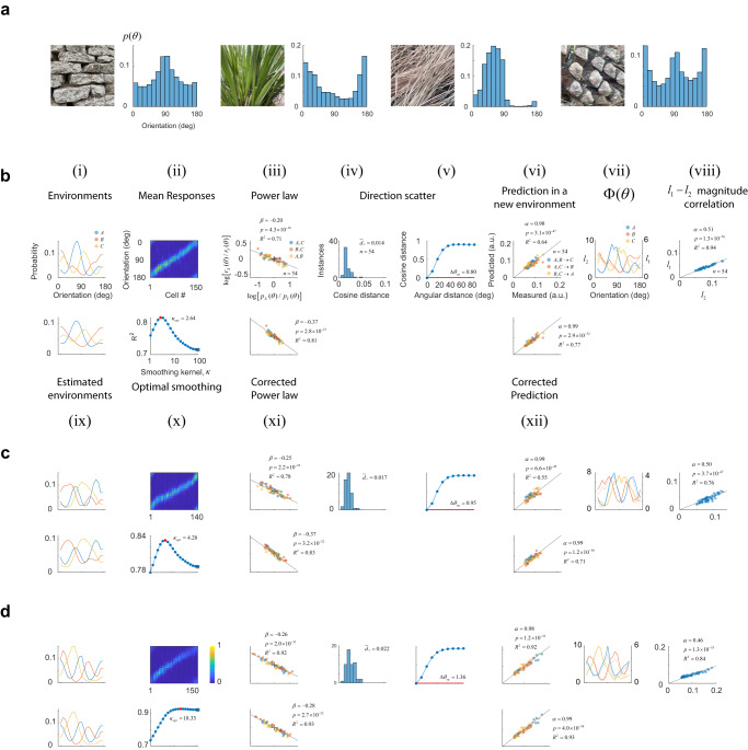
How do neural populations adapt to the time-varying statistics of sensory input? We used two-photon imaging to measure the activity of neurons in mouse primary visual cortex adapted to different sensory environments, each defined by a distinct probability distribution over a stimulus set. We find that two properties of adaptation capture how the population response to a given stimulus, viewed as a vector, changes across environments. First, the ratio between the response magnitudes is a power law of the ratio between the stimulus probabilities. Second, the response direction to a stimulus is largely invariant. These rules could be used to predict how cortical populations adapt to novel, sensory environments. Finally, we show how the power law enables the cortex to preferentially signal unexpected stimuli and to adjust the metabolic cost of its sensory representation to the entropy of the environment.

Fig. 1. Experimental protocol.

a Sessions included the presentation of three environments, A, B, and C each associated with a different distribution over a stimulus set. Stimulus sets were either sinusoidal gratings of different orientations or brief natural movie segments. b A session consisted of six blocks, each containing a unique permutation of all three environments. Each environment was presented for 5 min. Within an environment, stimuli were drawn from the corresponding distribution and flashed at a rate of 3/s. The presentation protocol was meant to mimic the changes of the retinal image during saccadic eye movements^,,,. A blank screen was shown for 1 min between environments. From one session to the next, the order of the permutations was randomized. c Each session began with a coarse retinotopic mapping, where we determined the average locations of receptive fields within different sectors of the field of view, numbered 1–9. The bottom panel shows the center of the receptive fields for each sector mapped on the computer monitor. The background image represents the aggregate receptive field of the entire field of view. The red circle denotes its center. The dashed circle represents the circular window used during visual stimulation.

Fig. 2. Characterizing adaptation in neural populations.

Each row (a–e) shows results from a different experiment. Each column (i–viii) depicts separate analyses. Axes are labeled in the top row (a) and, unless otherwise noted, they have the same scale in all other rows (b–e). Columns represent: i the distribution of orientations associated with each environment. ii Mean responses of cells to an orientation. Each column in the image represents a tuning curve. Cells have been arranged according to their preferred orientation. Responses are normalized to the maximum and displayed according to the colormap at the inset. iii Logarithmic plot of the ratios between probabilities versus the ratio between magnitudes across the three possible pairs of environments. Colors indicate the corresponding pairs. The solid line represents the best-fitting line to the data (without intercept). Fit statistics appear at the inset: $\beta$ estimated slope, $p$ is the statistical significance $\beta$, $R^2$ is the goodness of fit, and $n$ is the total number of data points (the degrees of freedom of the model is $n-1$). iv Distribution of cosine distance scatter. The mean value appears at the inset. v Calculation of the equivalent angular distance. The estimated value in each case is noted at the inset. vi Using the power law to predict magnitudes of population responses in a new environment. Best-fitting line (without intercept) is shown as a solid line. Fit statistics appear at the inset: $\alpha$ estimated slope, $p$ is the $p$ value of $\alpha$, $R^2$ is the goodness of fit, and $n$ is the total number of data points (the degrees of freedom of the model is $n-1$). Population magnitudes are in arbitrary units. vii Testing for population homeostasis. In the case of homeostasis, the function $\mathrm{\Phi }\left(\theta \right)\cong$ $p\left(\theta \right)r\left(\theta \right)$ should be constant (see Methods). Solid lines and left y-axis represent this calculation when the response magnitude is the $l_2$ norm. Dashed lines and right y-axis show the result if the magnitude is defined as the $l_1$ norm. viii Correlation between the $l_2$ and $l_1$ norms across stimuli and environments. Norms are in arbitrary units. Solid line represents best linear fit (without intercept). Fit statistics appear at the inset: $\beta$ estimated slope, $p$ is the statistical significance $\beta$, $R^2$ is the goodness of fit, and $n$ is the total number of data points (the degrees of freedom of the model is $n-1$).

Fig. 3. Experimental results using peaked distributions.

Each panel (a, b) shows the result of one experiment. The top row in the panel is organized as in Fig. 2 and it shows: i the distribution of orientations, ii mean responses, iii ratios between probabilities versus the ratio between magnitudes across the three possible pairs of environments in double logarithmic coordinates. iv Distribution of cosine distance scatter, v equivalent angular distance, vi predictions of magnitudes of population responses in a new environment using the power law, vii test of population homeostasis, and viii correlation between $l_2$ and $l_2$ responses across all conditions. The bottom rows depict: ix distributions obtained after smoothing the actual probabilities in (i) with the optimal von Mises kernel with concentration ${\kappa }_{opt}$, x goodness of fit ($R^2$) as a function of the smoothing parameter $\kappa$. The curve has an inverted U-shape with the maximum goodness of fit, shown by the red circle, attained at an intermediate value, while the open square represents the outcome without smoothing, xi restoration of the power law under the assumption the cortex relies on a smoothed estimate of the actual probabilities, and xii predictions using the power law relationship derived from (xi).

Fig. 4. Testing the rules of adaptation using orientation distributions drawn from natural scenes.

a Orientation distributions in natural image patches photographed by the authors on the UCLA campus. b–d Results using naturalistic environments. The panels are formatted exactly as Fig. 3, showing: i the distribution of orientations, ii mean responses, iii ratios between probabilities versus the ratio between magnitudes across the three possible pairs of environments in double logarithmic coordinates, iv Distribution of cosine distance scatter, v equivalent angular distance, vi predictions of magnitudes of population responses in a new environment using the power law, vii test of population homeostasis, and viii correlation between $l_2$ and $l_2$ responses across all conditions. The bottom rows depict: ix distributions obtained after smoothing the actual probabilities in (i) with the optimal von Mises kernel with concentration ${\kappa }_{opt}$, x goodness of fit ($R^2$) as a function of the smoothing parameter $\kappa$. The curve has an inverted U-shape with the maximum goodness of fit attained at an intermediate value, x restoration of the power law under the assumption the cortex relies on a smoothed estimate of the actual probabilities, and xii predictions using the power law relationship derived from (xi).

Fig. 5. Testing the rules of adaptation using movie sequences.

Each panel (a–c) shows the results obtained in separate experiments. Each row has the same layout. i Movie clips were assigned ID from 1 to 18 in a random order. Environments were defined using the same type of distributions used in the experiments described in Fig. 4ii, Direction scatter, expressed in terms of the cosine distance, is shown by the orange bars. This is the same calculation shown in Figs. 2–4(iv) for sinusoidal grating data. The blue bars show a histogram of cosine distances between the mean population responses evoked by pairs of movie clips, iii ratios between probabilities versus the ratio between magnitudes across the 3 possible pairs of environments in double logarithmic coordinates, iv scatterplot of predictions of the magnitudes of population responses in a new environment using the power law versus measured values, v test of population homeostasis, and vi correlation between the $l_2$ and $l_1$ population norms across stimuli and environments.

Fig. 6. Dynamics of adaptation and adaptation of metabolic cost to stimulus entropy.

a, b Modulation of response magnitude by a stimulus with orientation $\mathrm{\Delta }\theta$ away, shown $T$ s earlier in the sequence. Adaptation is fast—stimuli presented beyond 2 s into the past have no influence on the population response. b Same data as in (a), for $\mathrm{\Delta }\theta =0\mathrm{deg}$ and $\mathrm{\Delta }\theta =90\mathrm{deg}$ with solid lines showing exponential fits to the data. We refer to ${\tau }_d$ as the depletion time constant and ${\tau }_r$ as the recovery time constant. The terms are used for convenience and are not meant to imply we know the mechanism behind adaptation is synaptic depression. c Modulatory effect of an immediately preceding stimulus jointly as a function of relative shifts in orientation and spatial phase. The data for $\mathrm{\Delta }\theta =0\mathrm{deg}$ show that adaptation is sensitive to spatial phase. d Dependence of metabolic cost as a function of entropy in environments defined by von Mises distribution with concentration parameter $\kappa \in \left[\mathrm{0,\; 10}\right]$. Each curve is labeled with the corresponding exponent, $\beta$. Solid curves represent the range of experimentally observed exponents. e Magnitude of the modulation in metabolic cost with entropy (measured by the difference between maximum and minimum values in panel (d)) as a function of power law exponent (solid black curve), and linearity of the cost versus entropy relationship as assessed by the $R^2$ statistic to the linear fits of the curves in panel (d) (red, solid curve). f Average population magnitudes for populations adapting with different exponents for the case of a von Mises distribution with $\kappa =1.2$. Solid curves represent the compensation expected for the range of exponents in our experimental data. Population magnitudes are assumed to equal one in response to individual stimuli.

Fig. 7. Consistency of direction invariance with shifts in preferred orientation and tuning curve skewness.

a Responses of a homogenous population in a uniform environment. b Modulation function evoked by an adaptor at 90°. Each row in (a) is multiplied by its corresponding gain to yield the responses of the population under adaptation in (c. d), Examples of a few tuning curves (columns of (c)) under adaptation. Solid curves show two tuning curves near the adaptor. The flanks of the tuning curves closer to the adaptor fall more rapidly than those facing away, shifting their preferred orientations. e Shifts in the preferred orientation of tuning curves under adaptation relative to the uniform environment. f Circular skewness of tuning curves after adaptation.

References

1. Clifford CW, et al. Visual adaptation: neural, psychological and computational aspects. Vision Res. 2007;47:3125–3131. doi: 10.1016/j.visres.2007.08.023. - DOI - PubMed
1. Webster, M. A. Adaptation and visual coding. J. Vis.10.1167/11.5.3 (2011). - PMC - PubMed
1. Kohn A. Visual adaptation: physiology, mechanisms, and functional benefits. J. Neurophysiol. 2007;97:3155–3164. doi: 10.1152/jn.00086.2007. - DOI - PubMed
1. Whitmire CJ, Stanley GB. Rapid sensory adaptation redux: a circuit perspective. Neuron. 2016;92:298–315. doi: 10.1016/j.neuron.2016.09.046. - DOI - PMC - PubMed
1. Wark B, Lundstrom BN, Fairhall A. Sensory adaptation. Curr. Opin. Neurobiol. 2007;17:423–429. doi: 10.1016/j.conb.2007.07.001. - DOI - PMC - PubMed
Publication types