Scaling Exponents of Time Series Data: A Machine Learning Approach

Abstract

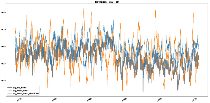
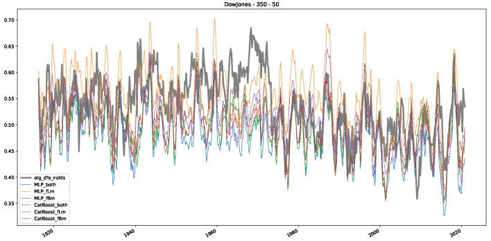
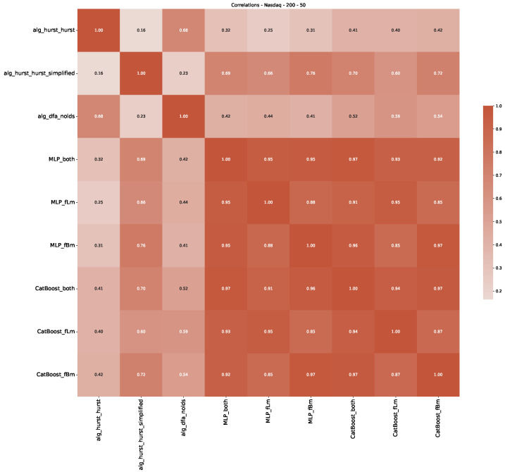
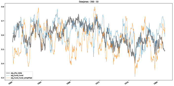
In this study, we present a novel approach to estimating the Hurst exponent of time series data using a variety of machine learning algorithms. The Hurst exponent is a crucial parameter in characterizing long-range dependence in time series, and traditional methods such as Rescaled Range (R/S) analysis and Detrended Fluctuation Analysis (DFA) have been widely used for its estimation. However, these methods have certain limitations, which we sought to address by modifying the R/S approach to distinguish between fractional Lévy and fractional Brownian motion, and by demonstrating the inadequacy of DFA and similar methods for data that resembles fractional Lévy motion. This inspired us to utilize machine learning techniques to improve the estimation process. In an unprecedented step, we train various machine learning models, including LightGBM, MLP, and AdaBoost, on synthetic data generated from random walks, namely fractional Brownian motion and fractional Lévy motion, where the ground truth Hurst exponent is known. This means that we can initialize and create these stochastic processes with a scaling Hurst/scaling exponent, which is then used as the ground truth for training. Furthermore, we perform the continuous estimation of the scaling exponent directly from the time series, without resorting to the calculation of the power spectrum or other sophisticated preprocessing steps, as done in past approaches. Our experiments reveal that the machine learning-based estimators outperform traditional R/S analysis and DFA methods in estimating the Hurst exponent, particularly for data akin to fractional Lévy motion. Validating our approach on real-world financial data, we observe a divergence between the estimated Hurst/scaling exponents and results reported in the literature. Nevertheless, the confirmation provided by known ground truths reinforces the superiority of our approach in terms of accuracy. This work highlights the potential of machine learning algorithms for accurately estimating the Hurst exponent, paving new paths for time series analysis. By marrying traditional finance methods with the capabilities of machine learning, our study provides a novel contribution towards the future of time series data analysis.

Keywords: Hurst exponent; artificial intelligence; complexity; machine learning; regression analysis; scaling exponent.

Figure A1

Plots depicting the different scaling behaviors of fractional Lévy motion with varying $\alpha$, for a fixed scaling exponent of $H=0.25$.

Figure A2

Plots depicting the different scaling behaviors of fractional Lévy motion with varying $\alpha$, for a fixed scaling exponent of $H=0.5$.

Figure A3

Plots depicting the different scaling behaviors of fractional Lévy motion with varying $\alpha$, for a fixed scaling exponent of $H=0.75$.

Figure A4

Plot depicting the time-varying DFA and Hurst exponents, as well as the predictions from trained machine learning models, using a 200-day input window and a 10-day step size between windows for the Dow Jones daily close values.

Figure A5

Plot depicting the time-varying DFA and Hurst exponents, using a 200-day input window and a 10-day step size between windows for the Dow Jones daily close values.

Figure A6

Plot depicting the time-varying DFA and predictions from all trained machine learning models, using a 200-day input window and a 10-day step size between windows for the Dow Jones daily close values.

Figure A7

Plot depicting the time-varying DFA and Hurst exponents, as well as the predictions from all trained machine learning models, using a 200-day input window and a 50-day step size between windows for the Dow Jones daily close values.

Figure A8

Plot depicting the time-varying DFA and Hurst exponents, using a 200-day input window and a 50-day step size between windows for the Dow Jones daily close values.

Figure A9

Plot depicting the time-varying DFA and predictions from all trained machine learning models, using a 200-day input window and a 50-day step size between windows for the Dow Jones daily close values.

Figure A10

Correlation plot showing the relationships between the DFA, various Hurst exponent estimation methods, and the predictions of all trained machine learning models for the Dow Jones index, using a 200-day rolling window size and a step size of 50 days for the Dow Jones daily close values.

Figure A11

Plot depicting the time-varying DFA and Hurst exponents, as well as the predictions from all trained machine learning models, using a 350-day input window and a 10-day step size between windows for the Dow Jones daily close values.

Figure A12

Plot depicting the time-varying DFA and Hurst exponents, using a 350-day input window and a 10-day step size between windows for the Dow Jones daily close values.

Figure A13

Plot depicting the time-varying DFA and predictions from all trained machine learning models, using a 350-day input window and a 10-day step size between windows for the Dow Jones daily close values.

Figure A14

Correlation plot showing the relationships between the DFA, various Hurst exponent estimation methods, and the predictions of all trained machine learning models for the Dow Jones index, using a 350-day rolling window size and a step size of 10 days for the Dow Jones daily close values.

Figure A15

Plot depicting the time-varying DFA and Hurst exponents, as well as the predictions from all trained machine learning models, using a 350-day input window and a 50-day step size between windows for the Dow Jones daily close values.

Figure A16

Plot depicting the time-varying DFA and Hurst exponents, using a 350-day input window and a 50-day step size between windows for the Dow Jones daily close values.

Figure A17

Plot depicting the time-varying DFA and predictions from all trained machine learning models, using a 350-day input window and a 50-day step size between windows for the Dow Jones daily close values.

Figure A18

Correlation plot showing the relationships between the DFA, various Hurst exponent estimation methods, and the predictions of all trained machine learning models for the Dow Jones index, using a 350-day rolling window size and a step size of 50 days for the Dow Jones daily close values.

Figure A19

Plot depicting the time-varying DFA and Hurst exponents, as well as the predictions from all trained machine learning models, using a 200-day input window and a 10-day step size between windows for the S&P500 daily close values.

Figure A20

Plot depicting the time-varying DFA and Hurst exponents, using a 200-day input window and a 10-day step size between windows for the S&P500 daily close values.

Figure A21

Plot depicting the time-varying DFA and predictions from all trained machine learning models, using a 200-day input window and a 10-day step size between windows for the S&P500 daily close values.

Figure A22

Correlation plot showing the relationships between the DFA, various Hurst exponent estimation methods, and the predictions of all trained machine learning models for the Dow Jones index, using a 200-day rolling window size and a step size of 10 days for the S&P500 daily close values.

Figure A23

Plot depicting the time-varying DFA and Hurst exponents, as well as the predictions from all trained machine learning models, using a 200-day input window and a 50-day step size between windows for the S&P500 daily close values.

Figure A24

Plot depicting the time-varying DFA and Hurst exponents, using a 200-day input window and a 50-day step size between windows for the S&P500 daily close values.

Figure A25

Plot depicting the time-varying DFA and predictions from all trained machine learning models, using a 200-day input window and a 50-day step size between windows for the S&P500 daily close values.

Figure A26

Correlation plot showing the relationships between the DFA, various Hurst exponent estimation methods, and the predictions of all trained machine learning models for the Dow Jones index, using a 200-day rolling window size and a step size of 50 days for the S&P500 daily close values.

Figure A27

Plot depicting the time-varying DFA and Hurst exponents, as well as the predictions from all trained machine learning models, using a 350-day input window and a 10-day step size between windows for the S&P500 daily close values.

Figure A28

Plot depicting the time-varying DFA and Hurst exponents, using a 350-day input window and a 10-day step size between windows for the S&P500 daily close values.

Figure A29

Plot depicting the time-varying DFA and predictions from all trained machine learning models, using a 350-day input window and a 10-day step size between windows for the S&P500 daily close values.

Figure A30

Correlation plot showing the relationships between the DFA, various Hurst exponent estimation methods, and the predictions of all trained machine learning models for the Dow Jones index, using a 350-day rolling window size and a step size of 10 days for the S&P500 daily close values.

Figure A31

Plot depicting the time-varying DFA and Hurst exponents, as well as the predictions from all trained machine learning models, using a 350-day input window and a 50-day step size between windows for the S&P500 daily close values.

Figure A32

Plot depicting the time-varying DFA and Hurst exponents, using a 350-day input window and a 50-day step size between windows for the S&P500 daily close values.

Figure A33

Plot depicting the time-varying DFA and predictions from all trained machine learning models, using a 350-day input window and a 50-day step size between windows for the S&P500 daily close values.

Figure A34

Correlation plot showing the relationships between the DFA, various Hurst exponent estimation methods, and the predictions of all trained machine learning models for the Dow Jones index, using a 350-day rolling window size and a step size of 50 days for the S&P500 daily close values.

Figure A35

Plot depicting the time-varying DFA and Hurst exponents, as well as the predictions from all trained machine learning models, using a 200-day input window and a 10-day step size between windows for the NASDAQ daily close values.

Figure A36

Plot depicting the time-varying DFA and Hurst exponents, using a 200-day input window and a 10-day step size between windows for the NASDAQ daily close values.

Figure A37

Plot depicting the time-varying DFA and predictions from all trained machine learning models, using a 200-day input window and a 10-day step size between windows for the NASDAQ daily close values.

Figure A38

Correlation plot showing the relationships between the DFA, various Hurst exponent estimation methods, and the predictions of all trained machine learning models for the Dow Jones index, using a 200-day rolling window size and a step size of 10 days for the NASDAQ daily close values.

Figure A39

Plot depicting the time-varying DFA and Hurst exponents, as well as the predictions from all trained machine learning models, using a 200-day input window and a 50-day step size between windows for the NASDAQ daily close values.

Figure A40

Plot depicting the time-varying DFA and Hurst exponents, using a 200-day input window and a 50-day step size between windows for the NASDAQ daily close values.

Figure A41

Plot depicting the time-varying DFA and predictions from all trained machine learning models, using a 200-day input window and a 50-day step size between windows for the NASDAQ daily close values.

Figure A42

Correlation plot showing the relationships between the DFA, various Hurst exponent estimation methods, and the predictions of all trained machine learning models for the Dow Jones index, using a 200-day rolling window size and a step size of 50 days for the NASDAQ daily close values.

Figure A43

Plot depicting the time-varying DFA and Hurst exponents, as well as the predictions from all trained machine learning models, using a 350-day input window and a 10-day step size between windows for the NASDAQ daily close values.

Figure A44

Plot depicting the time-varying DFA and Hurst exponents, using a 350-day input window and a 10-day step size between windows for the NASDAQ daily close values.

Figure A45

Plot depicting the time-varying DFA and predictions from all trained machine learning models, using a 350-day input window and a 10-day step size between windows for the NASDAQ daily close values.

Figure A46

Correlation plot showing the relationships between the DFA, various Hurst exponent estimation methods, and the predictions of all trained machine learning models for the Dow Jones index, using a 350-day rolling window size and a step size of 10 days for the NASDAQ daily close values.

Figure A47

Plot depicting the time-varying DFA and Hurst exponents, as well as the predictions from all trained machine learning models, using a 350-day input window and a 50-day step size between windows for the NASDAQ daily close values.

Figure A48

Plot depicting the time-varying DFA and Hurst exponents, using a 350-day input window and a 50-day step size between windows for the NASDAQ daily close values.

Figure A49

Plot depicting the time-varying DFA and predictions from all trained machine learning models, using a 350-day input window and a 50-day step size between windows for the NASDAQ daily close values.

Figure A50

Correlation plot showing the relationships between the DFA, various Hurst exponent estimation methods, and the predictions of all trained machine learning models for the Dow Jones index, using a 350-day rolling window size and a step size of 50 days for the NASDAQ daily close values.

Figure 1

This figure presents a correlation plot illustrating the relationship between predicted and actual values in estimating the Hurst exponent for fractional Brownian motion data. The horizontal axis represents the true Hurst values, while the vertical axis shows the predicted values by various algorithms. These are the results for a window length of 100 data points from Table 2 and Table 3.

Figure 2

Time series plots for the daily closing values of the assets used in our study, i.e., Dow Jones, S&P 500 and NASDAQ. On the left side, we see regular plots, and on the right side, the y-axis is in a logarithmic scale, illustrating the relative changes in the value of the assets. We studied the Dow Jones from 12 December 1914 to 15 December 2020, S&P500 goes from 30 December 1927 to the 4 November 2020 and for the NASDAQ the studied period starts on the 5 February 1972 and ends on the 16 April 2021.

Figure 2

Time series plots for the daily closing values of the assets used in our study, i.e., Dow Jones, S&P 500 and NASDAQ. On the left side, we see regular plots, and on the right side, the y-axis is in a logarithmic scale, illustrating the relative changes in the value of the assets. We studied the Dow Jones from 12 December 1914 to 15 December 2020, S&P500 goes from 30 December 1927 to the 4 November 2020 and for the NASDAQ the studied period starts on the 5 February 1972 and ends on the 16 April 2021.

Figure 2

Time series plots for the daily closing values of the assets used in our study, i.e., Dow Jones, S&P 500 and NASDAQ. On the left side, we see regular plots, and on the right side, the y-axis is in a logarithmic scale, illustrating the relative changes in the value of the assets. We studied the Dow Jones from 12 December 1914 to 15 December 2020, S&P500 goes from 30 December 1927 to the 4 November 2020 and for the NASDAQ the studied period starts on the 5 February 1972 and ends on the 16 April 2021.

Figure 3

The scaling analysis in the graph offers a comparative view between the three asset datasets: Dow Jones, NASDAQ, and S&P500, as well as fractional Brownian motion. Furthermore, three distinct fractional Lévy motions with a scaling exponent of $H=0.5$ are also presented. Each fractional Lévy motion depicted has a unique $\alpha$ value (refer to Section 3.1 for more specifics). Note that the R/S ratio displayed is the average R/S ratio, as outlined in Equation (17). To better illustrate the distinctions among the various time series data, we have also provided a zoomed-in view of the final section of the analysis (in terms of the scale $\tau$) in the upper left corner. While this close-up does not include the fractional Brownian motion, it successfully emphasizes the slight differences between the financial time series data, which are otherwise densely clustered.

Figure 4

Plot depicting the time-varying DFA and Hurst exponents, as well as the predictions from all trained machine learning models, using a 200-day input window and a 10-day step size between windows, close up for the years 1960–1980.

Figure 5

Plot depicting the time-varying DFA and Hurst exponents, using a 200-day input window and a 10-day step size between windows, close up for the years 1960–1980.

Figure 6

Plot depicting the time-varying DFA and predictions from all trained machine learning models, using a 200-day input window and a 10-day step size between windows, close up for the years 1960–1980.

Figure 7

Correlation plot showing the relationships between the DFA, various Hurst exponent estimation methods, and the predictions of all trained machine learning models for the Dow Jones index, using a 200-day rolling window size and a step size of 10 days, close up for the years 1960–1980.

References

1. Mandelbrot B.B., Wallis J.R. Robustness of the rescaled range R/S in the measurement of noncyclic long run statistical dependence. Water Resour. Res. 1969;5:967–988. doi: 10.1029/WR005i005p00967. - DOI
1. Peters E.E. Fractal Market Analysis: Applying Chaos Theory to Investment and Economics. J. Wiley & Sons; New York, NY, USA: 1994. Wiley Finance Editions.
1. Turcotte D.L. Fractals and Chaos in Geology and Geophysics. 2nd ed. Cambridge University Press; Cambridge, UK: 1997. - DOI
1. Ivanov P.C., Amaral L.A.N., Goldberger A.L., Havlin S., Rosenblum M.G., Struzik Z.R., Stanley H.E. Multifractality in human heartbeat dynamics. Nature. 1999;399:461–465. doi: 10.1038/20924. - DOI - PubMed
1. Hurst H., Black R., Sinaika Y. Long-Term Storage in Reservoirs: An Experimental Study. Constable; London, UK: 1965.
LinkOut - more resources