Segmentation of cellular ultrastructures on sparsely labeled 3D electron microscopy images using deep learning

Abstract

Focused ion beam-scanning electron microscopy (FIB-SEM) images can provide a detailed view of the cellular ultrastructure of tumor cells. A deeper understanding of their organization and interactions can shed light on cancer mechanisms and progression. However, the bottleneck in the analysis is the delineation of the cellular structures to enable quantitative measurements and analysis. We mitigated this limitation using deep learning to segment cells and subcellular ultrastructure in 3D FIB-SEM images of tumor biopsies obtained from patients with metastatic breast and pancreatic cancers. The ultrastructures, such as nuclei, nucleoli, mitochondria, endosomes, and lysosomes, are relatively better defined than their surroundings and can be segmented with high accuracy using a neural network trained with sparse manual labels. Cell segmentation, on the other hand, is much more challenging due to the lack of clear boundaries separating cells in the tissue. We adopted a multi-pronged approach combining detection, boundary propagation, and tracking for cell segmentation. Specifically, a neural network was employed to detect the intracellular space; optical flow was used to propagate cell boundaries across the z-stack from the nearest ground truth image in order to facilitate the separation of individual cells; finally, the filopodium-like protrusions were tracked to the main cells by calculating the intersection over union measure for all regions detected in consecutive images along z-stack and connecting regions with maximum overlap. The proposed cell segmentation methodology resulted in an average Dice score of 0.93. For nuclei, nucleoli, and mitochondria, the segmentation achieved Dice scores of 0.99, 0.98, and 0.86, respectively. The segmentation of FIB-SEM images will enable interpretative rendering and provide quantitative image features to be associated with relevant clinical variables.

Keywords: cell boundary; deep neural network; electron microscopy; segmentation; subcellular ultrastructure.

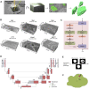
FIGURE 1

(A) FIB-SEM-to-volume rendering workflow. The FIB source sequentially slices a few nanometers from the sample to expose a fresh surface for subsequent imaging using the electron beam. An image stack is acquired, and after image alignment and cropping, a small subset of the stack of images was segmented manually to generate a training set for the deep learning model. Once trained, the deep learning model is used to predict segmentation masks for the rest of the images in the stack. These predictions are used to create volume renderings for the examination of 3D ultrastructural properties. (B) Six FIB-SEM datasets and their sizes. The 3D FIB-SEM volumes collected from the biopsy samples Bx1, Bx2, and Bx4 acquired from a patient with metastatic breast ductal carcinoma, two biopsy samples (PTT and PDAC) acquired from two patients with pancreatic ductal adenocarcinoma, and a microspheroid prepared using a breast cancer cell line (MCF7). (C) Residual block used in ResUNet. BN stands for batch normalization, and ReLU stands for rectified linear unit. X _l and X _l+1 are the input and output features for the residual layer l, respectively, and F represents the residual function. (D) ResUNet architecture. Input size is written on the side of each box. The number of feature maps in each residual layer is written on top of each box. (E) Illustration of the net volume and filled volume used in the fenestrated volume percentage measure (3D volume is represented as a 2D image) and (F) illustration of distances d _cc and d _s used in proximity of the nucleolus to the nuclear membrane measure.

FIGURE 2

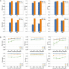
Nucleus and nucleolus segmentation performance. (A) Effect of image tile size (context window). Segmentation performances for nuclei (top row) and nucleoli (bottom row) using different input tile sizes measured by the Dice score (first column), precision (second column), and recall (third column) on the Bx1 and PTT datasets. The blue bar represents the results of training the network directly on the image tiles of size 512 × 512 pixels from the FIB-SEM images. The orange bar represents the results of training the network on the image tiles of size 2,048 × 2,048 pixels downsampled to 512 × 512 pixels, which provide larger contextual information. Each error bar represents 10 separate experiments in which a new model was trained from scratch using the specified number of training images. (B) Effect of training set size. Segmentation performances for nuclei (top row) and nucleoli (bottom row) using different training set sizes, measured by the Dice score (first column), precision (second column), and recall (third column) on PTT (blue), Bx1 (orange), and Bx2 (green) datasets. For each dataset, the performance was evaluated over training set sizes of 7, 10, 15, 25, and 50 in order to find the minimum number of images required to generate accurate segmentation. Each error bar represents the mean and standard deviation of results obtained from 10 separate experiments in which a new model was trained from scratch using the specified number of training images.

FIGURE 3

Nucleus and nucleolus volume renderings and nucleolus segmentation results. (A) Volume renderings showing the 3D structure of ground truth masks and predicted segmentation masks for PTT, Bx1, and Bx2 datasets. (B) Volume rendering showing the 3D structure of predicted segmentation masks for the Bx4 dataset. (C) Representative qualitative results showing input images (first column), ground truth (second column), and predicted nucleoli (third column) for PTT (first row), Bx1 (second row), and Bx2 (third row) datasets. (D) Volume renderings of the fenestrations in the nucleoli of PTT, Bx1, Bx2, and Bx4 datasets.

FIGURE 4

Cell and organelle segmentation results on Bx1, Bx2, PDAC, and MCF7 datasets. Qualitative results showing input images (first row) overlaid with nucleus (yellow), nucleolus (red), mitochondrion (pink), endosome (white), lysosome (black), and cell segmentation (random colors) on ground truth masks (second row) and predicted segmentation masks (third row) for (A) Bx1 (B) Bx2, (C) PDAC, and (D) MCF7 datasets.

FIGURE 5

Nucleus and nucleolus segmentation results on PTT and Bx4 datasets. (A) Representative qualitative results showing input images (top row) overlaid with nucleus (green) and nucleolus (red) ground truth masks (middle row) and predicted nucleus (yellow) and nucleolus (pink) segmentation masks (bottom row) for the PTT dataset. (B) Representative qualitative results showing input images (top row) overlaid with predicted nucleus (yellow) and nucleolus (pink) segmentation masks (bottom row) for the Bx4 dataset. All 19 slices from the Bx4 dataset that had nucleolus labels were employed in the training of ResUNet, resulting in the possibility of conducting only a qualitative comparison. Numbers in the lower right-hand corner of images indicate the slice position of the image in the full image stack. Scale: horizontal image width = 25 μm.

FIGURE 6

Nucleus segmentation performance using ResUNet, TransUNet, and SETR. Segmentation performances for nuclei using different input tile sizes measured by the Dice score (first column), precision (second column), and recall (third column) on the PTT, Bx1, and Bx2 datasets. The lighter bar represents the results of training the network directly on the tiles of size 512 × 512 pixels from the FIB-SEM images. The darker bar represents the results of training the network on image tiles of size 2,048 × 2,048 pixels downsampled to 512 × 512 pixels, which provide larger contextual information.

FIGURE 7

Cell segmentation results on the Bx1 dataset. Red boxes represent regions where the cells could not be separated accurately, and blue box represents regions where the cell protrusions are not segmented accurately. Representative qualitative results showing (A) input image, (B) ground truth segmentation (a few cells are not labeled in the ground truth), (C) segmentation of cells using a cell-interior mask alone, (D) segmentation of cells using a cell-interior mask and boundary predictions from the segmentation model, (E) segmentation of cells using optical flow alone, (F) segmentation of cells by overlaying boundaries propagated using optical flow on the cell-interior mask obtained from the segmentation model to separate cells, (G) segmentation of cells by selectively combining the optical flow boundary estimate with the boundary estimated from the segmentation model, and (H) segmentation of cells by propagating boundaries estimated in the previous frame using optical flow and combining with the boundary estimated from the segmentation model for the Bx1 dataset.

FIGURE 8

Cell segmentation results on the Bx2 dataset. Red boxes represent regions where the cells could not be separated accurately, and blue boxes represent regions where the cell protrusions are not segmented accurately. Representative qualitative results showing (A) input image, (B) ground truth segmentation (a few cells are not labeled in the ground truth), (C) segmentation of cells using a cell-interior mask alone, (D) segmentation of cells using a cell-interior mask and boundary predictions from the segmentation model, (E) segmentation of cells using optical flow alone, (F) segmentation of cells by overlaying boundaries propagated using optical flow on a cell-interior mask obtained from the segmentation model to separate cells, (G) segmentation of cells by selectively combining the optical flow boundary estimate with the boundary estimated from the segmentation model, and (H) segmentation of cells by propagating boundaries estimated in the previous frame using optical flow and combining with the boundary estimated from the segmentation model for the Bx2 dataset.

FIGURE 9

Volume rendering of a cell from the Bx2 dataset. Volume rendering of the (left to right) (A) ground truth, (B) cell segmented by using the watershed algorithm on the cell-interior mask from ResUNet, and (C) cell segmented by using the watershed algorithm on the cell-interior mask with boundary information from both ResUNet and optical flow.

FIGURE 10

(A–D) Volume renderings showing the FIB-SEM volume and the predicted cell and organelle segmentations in PDAC and MCF7 datasets. (E–H) Volume occupied by the predicted organelles for each cell in each dataset.

FIGURE 11

Morphological features extracted from nuclei and nucleoli. Solidity, sphericity, and circular variance measures for (A) nuclei and (B) nucleoli in PTT, Bx1, Bx2, and Bx4 datasets. (C) Percentage of the fenestrated volume in nucleoli and the proximity of nucleoli to the nuclear membrane for all datasets. Each dot represents the value of the feature for a nucleus or nucleolus.

FIGURE 12

Texture features extracted from nuclei and nucleoli. GLCM features (top row), pattern spectrum, and SZM features (bottom row) for (A) nuclei and (B) nucleoli in PTT, Bx1, Bx2, and Bx4 datasets. Each dot represents the value of the feature for a nucleus or nucleolus.

References

1. Abadi M., Barham P., Chen J., Chen Z., Davis A., Dean J., et al. (2016). “TensorFlow: a system for {Large-Scale} machine learning,” in 12th USENIX symposium on operating systems design and implementation (OSDI 16) (Savannah, GA, USA: ACM; ), 265–283.
1. Baba A. I., Câtoi C. (2007). “Tumor cell morphology,” in Comparative oncology (Bucuresti, România: The Publishing House of the Romanian Academy; ). - PubMed
1. Baghban R., Roshangar L., Jahanban-Esfahlan R., Seidi K., Ebrahimi-Kalan A., Jaymand M., et al. (2020). Tumor microenvironment complexity and therapeutic implications at a glance. Cell. Commun. Signal. 18, 59–19. 10.1186/s12964-020-0530-4 - DOI - PMC - PubMed
1. Barnes R., Lehman C., Mulla D. (2014). Priority-flood: an optimal depression-filling and watershed-labeling algorithm for digital elevation models. Comput. Geosciences 62, 117–127. 10.1016/j.cageo.2013.04.024 - DOI
1. Belevich I., Joensuu M., Kumar D., Vihinen H., Jokitalo E. (2016). Microscopy image browser: a platform for segmentation and analysis of multidimensional datasets. PLoS Biol. 14, e1002340. 10.1371/journal.pbio.1002340 - DOI - PMC - PubMed
LinkOut - more resources