What can entropy metrics tell us about the characteristics of ocular fixation trajectories?

Abstract

In this study, we provide a detailed analysis of entropy measures calculated for fixation eye movement trajectories from the three different datasets. We employed six key metrics (Fuzzy, Increment, Sample, Gridded Distribution, Phase, and Spectral Entropies). We calculate these six metrics on three sets of fixations: (1) fixations from the GazeCom dataset, (2) fixations from what we refer to as the "Lund" dataset, and (3) fixations from our own research laboratory ("OK Lab" dataset). For each entropy measure, for each dataset, we closely examined the 36 fixations with the highest entropy and the 36 fixations with the lowest entropy. From this, it was clear that the nature of the information from our entropy metrics depended on which dataset was evaluated. These entropy metrics found various types of misclassified fixations in the GazeCom dataset. Two entropy metrics also detected fixation with substantial linear drift. For the Lund dataset, the only finding was that low spectral entropy was associated with what we call "bumpy" fixations. These are fixations with low-frequency oscillations. For the OK Lab dataset, three entropies found fixations with high-frequency noise which probably represent ocular microtremor. In this dataset, one entropy found fixations with linear drift. The between-dataset results are discussed in terms of the number of fixations in each dataset, the different eye movement stimuli employed, and the method of eye movement classification.

Fig 1. Fixation durations across the three datasets.

In Fig 1 violin plots are presented representing the duration of fixations (in samples) across the three datasets. The durations between datasets were statistically significantly different. In Fig 1B we show the same plots after we had taken steps to equalize the fixation duration distributions across datasets.

Fig 2. Plot of the trajectory of the states thru the phase space from Table 5.

Fig 3. Explanatory plot for the fuzzy entropy.

In Fig 3A we have a fixation with high position change and relatively high FuzzEn. In Fig 3B we see the phase space reconstruction with the parameters τ = 1 and m = 2 for the fixation in Fig 3A and provide the membership degree for the trajectory in Fig 3B. In Fig 3C, we present a fixation with smaller position change and its phase space reconstruction in Fig 3D. In Fig 3E, we present a fixation with the lowest FuzzEn value and its 2-D trajectory in Fig 3F.

Fig 4. The Increment Entropy.

The top row illustrates 3 fixations with high IncrEn, the middle row illustrates fixations with intermediate IncrEn and the bottom row illustrates fixations with low IncrEn.

Fig 5. Explanatory plot for the Sample Entropy.

In Fig 5A we have a relatively chaotic fixation. In Fig 5B we see the phase space reconstruction with the parameters τ = 1 and m = 2 for the fixation in Fig 5A. In Fig 5C, we present a much less chaotic fixation and its 2-D fixation trajectory Fig 5D. In Fig 5E, we present a fixation with the lowest SampEn value and its reconstructed trajectory Fig 5F.

Fig 6. The gridded Distribution Entropy.

In Fig 6A–6C there are three examples of fixation when this entropy is high. In Fig 6G–6I there are three examples of fixation when this entropy is low. In Fig 6D–6F there are three examples of fixations with entropy values intermediate between the high values and low values.

Fig 7. The Poincare plot for the GridEn for each fixation is illustrated in Fig 6.

Each Poincare plot is divided into a 3-by-3 grid (9 squares), corresponding to the fixation with the same letter in Fig 6. In the right corner of each square, we present the number of points in that region. Fig 7A–7C are examples of fixations that exhibit a high value of GridEn because points on the Poincare plot are highly distributed across all nine regions. When points on the Poincare plots are mostly distributed across 2 (or 3) dominant regions, the corresponding trajectories will be characterized by an average value of GridEn (see Fig 7D–7F). In Fig 7G–7I there are three examples of fixations in which points are mainly located in one dominant region. This produces a low GridEn.

Fig 8. The Phase Entropy.

In this plot, we present the 9 fixations. The top row consists of examples with high PhasEn, the bottom row consists of examples with low PhasEn and the middle row consists of examples with intermediate PhasEn.

Fig 9. The Second Order Differences Plots (SODP) for each fixation illustrated in Fig 8.

The top row shows SODP plots for the 3 fixations previously illustrated with high PhasEn. The middle row displays 3 fixations with intermediate PhasEn, and the bottom row depicts 3 fixations with low PhasEn. For each fixation, the SODP is divided into 4 radial sectors. In the corner of each sector, we display the number of points contained within that sector. Fig 9A to.9C depict three examples of fixation where the SODP points are highly distributed across the four sectors. Fig 9D to.9F present three examples of fixation where the SODP points are less randomly distributed across the four sectors compared to the first three examples, but more randomly distributed than the last three examples. Finally, Fig 9G to.9I display three examples of fixation where the SODP points are predominantly located within a single dominant sector.

Fig 10. Explanatory plot for the Spectral Entropy.

The frequency plots have been scaled from 0 to 0.001 to better visualize the higher frequency estimates. In Fig 10A, we present a relatively chaotic fixation, and its corresponding frequency plot is shown in Fig 10B. The chart of normalized spectral density by frequency exhibits multiple levels, resulting in a high value of SpecEn. In Fig 10C, we present a fixation that is much less chaotic, leading to a narrower range of normalized density in the higher frequencies (refer to Fig 10D). In Fig 10E, we showcase a relatively smooth fixation, which is associated with very little variability in normalized density estimates in the upper frequencies (see Fig 10F).

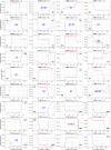
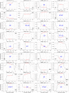
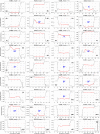
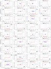
Fig 11. GazeCom dataset: 36 horizontal fixations with the highest GridEn values.

The fixations are plotted in red. There are 30 signal samples before and after each fixation. The entropy value is displayed above each fixation chart. The classification of each fixation is shown in blue in the middle of each fixation chart. The fixation at the top left has the highest entropy value. Note the common occurrence of fixations that start too late on this page.

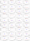
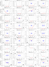
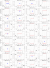
Fig 12. GazeCom dataset: 36 fixations with the lowest GridEn values.

See the caption of Fig 11 for more details. The fixation with the lowest entropy value is shown in the bottom right. Note that 23 fixations start with a corrective saccade (CS) on this page.

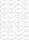
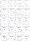
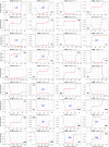
Fig 13. GazeCom dataset: 36 fixations with the lowest PhasEn values.

See the caption of Fig 11 for more details. Note that 14 fixations exhibit linear drift (LD) on this page.

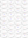
Fig 14. GazeCom dataset: 36 fixations with high SampEn values.

See the caption of Fig 11 for more details.

Fig 15. GazeCom dataset: 36 fixations with low SampEn values.

See the caption of Fig 11 for more details.

Fig 16. GazeCom dataset: 36 fixations with low IncrEn values.

See the caption of Fig 11 for more details.

Fig 17. GazeCom dataset: 36 fixations with high SpecEn values.

See the caption of Fig 11 for more details.

Fig 18. GazeCom dataset: 36 fixations with high FuzzEn values.

See the caption of Fig 11 for more details.

Fig 19. GazeCom dataset: 36 fixations with low FuzzEn values.

See the caption of Fig 11 for more details.

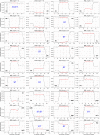
Fig 20. Lund dataset: 36 fixations with low SpecEn values.

See the caption of Fig 11 for more details.

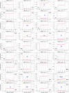
Fig 21. OK lab dataset: 36 fixations with high GridEn values.

See the caption of Fig 11 for more details.

Fig 22. OK lab dataset: 36 fixations with low SampEn values.

See the caption of Fig 11 for more details.

Fig 23. OK lab dataset: 36 fixations with low SpecEn values.

See the caption of Fig 11 for more details.

Fig 24. OK lab dataset: 36 fixations with high FuzzEn values.

See the caption of Fig 11 for more details.

References

1. Rigas I, Friedman L, Komogortsev O. Study of an Extensive Set of Eye Movement Features: Extraction Methods and Statistical Analysis. J Eye Mov Res. 2018;11(1). doi: 10.16910/jemr.11.1.3 - DOI - PMC - PubMed
1. Lohr D, Berndt SH, Komogortsev O. An Implementation of Eye Movement-Driven Biometrics in Virtual Reality. In: Proceedings of the 2018 ACM Symposium on Eye Tracking Research & Applications. ETRA’18. New York, NY, USA: Association for Computing Machinery; 2018. p. 1–3. Available from: 10.1145/3204493.3208333. - DOI
1. Friedman L, Stern HS, Price LR, Komogortsev OV. Why Temporal Persistence of Biometric Features, as Assessed by the Intraclass Correlation Coefficient, Is So Valuable for Classification Performance. Sensors. 2020;20(16). doi: 10.3390/s20164555 - DOI - PMC - PubMed
1. Griffith HK, Komogortsev OV. Texture Feature Extraction From Free-Viewing Scan Paths Using Gabor Filters With Downsampling. In: ACM Symposium on Eye Tracking Research and Applications. ETRA’20 Adjunct. New York, NY, USA: Association for Computing Machinery; 2020. p. 1–3. Available from: 10.1145/3379157.3391423. - DOI
1. Friedman L, Nixon MS, Komogortsev OV. Method to assess the temporal persistence of potential biometric features: Application to oculomotor, gait, face and brain structure databases. PLOS ONE. 2017;12:1–42. doi: 10.1371/journal.pone.0178501 - DOI - PMC - PubMed