A global dataset on phosphorus in agricultural soils

Abstract

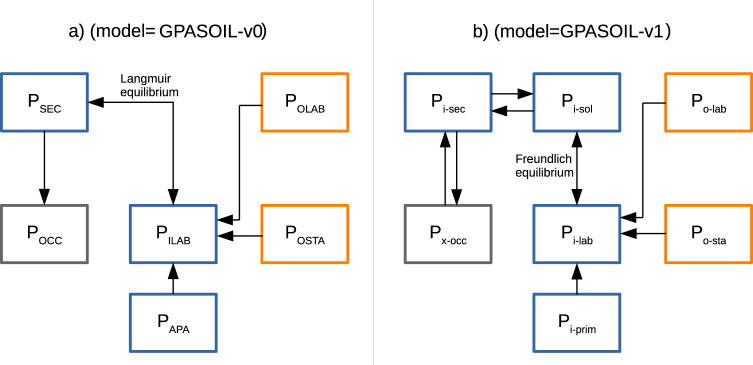
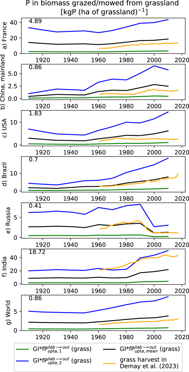
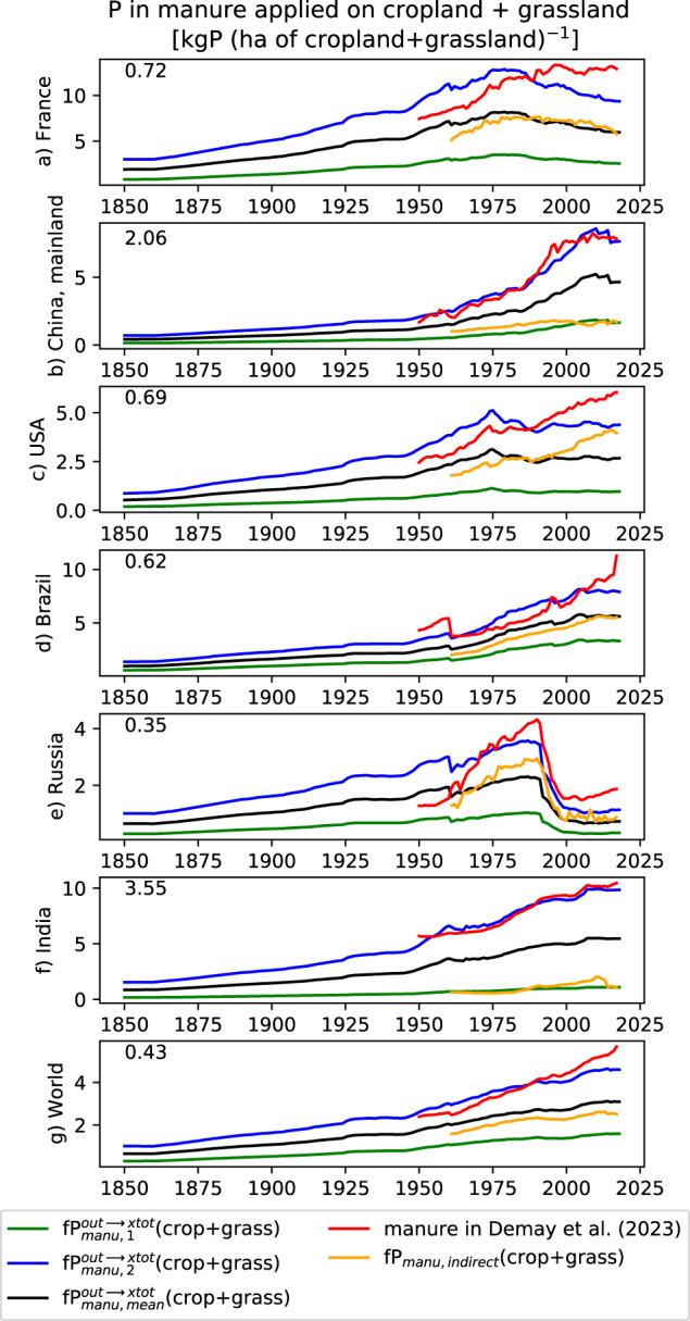
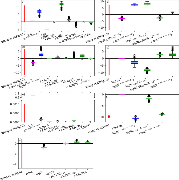
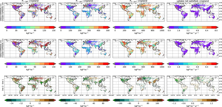
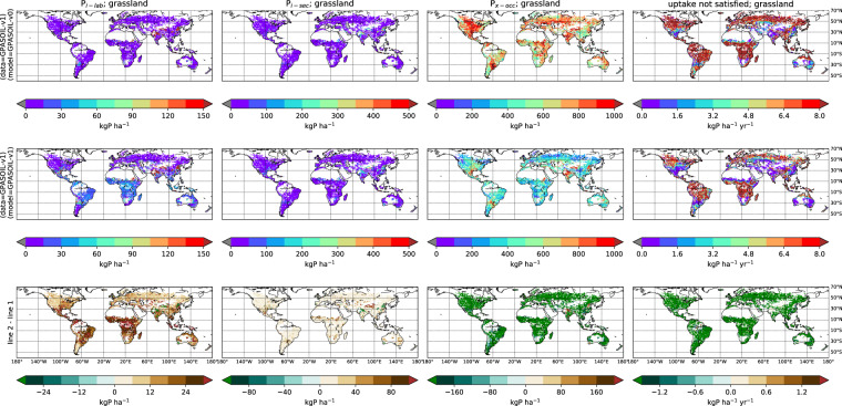
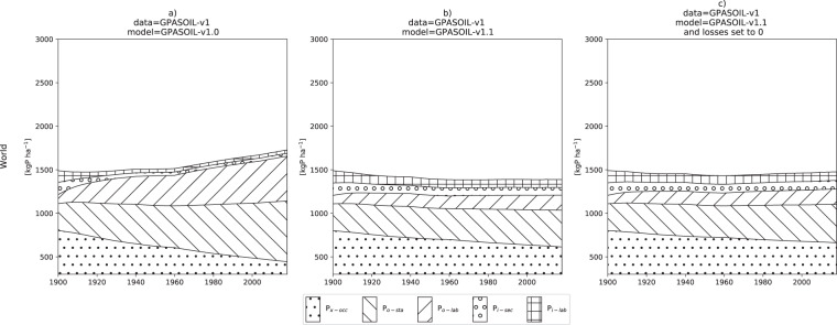
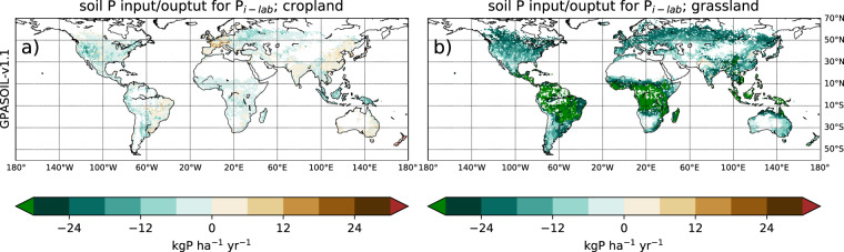
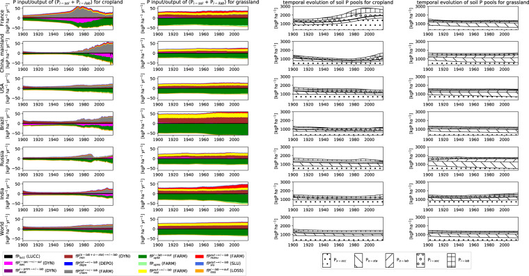
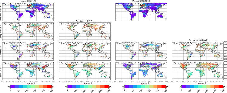
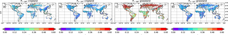
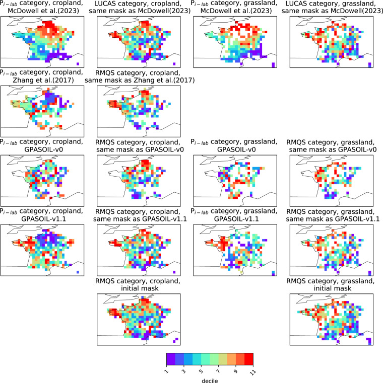
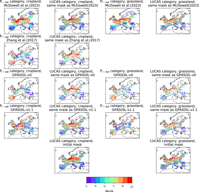
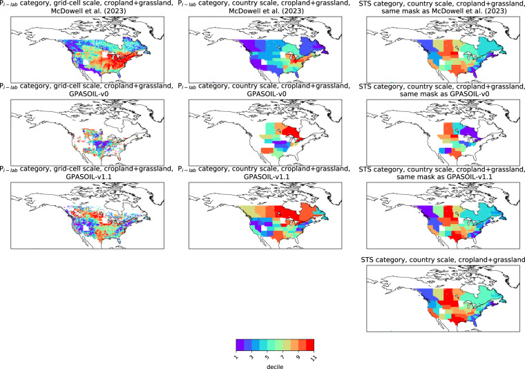
Numerous drivers such as farming practices, erosion, land-use change, and soil biogeochemical background, determine the global spatial distribution of phosphorus (P) in agricultural soils. Here, we revised an approach published earlier (called here GPASOIL-v0), in which several global datasets describing these drivers were combined with a process model for soil P dynamics to reconstruct the past and current distribution of P in cropland and grassland soils. The objective of the present update, called GPASOIL-v1, is to incorporate recent advances in process understanding about soil inorganic P dynamics, in datasets to describe the different drivers, and in regional soil P measurements for benchmarking. We trace the impact of the update on the reconstructed soil P. After the update we estimate a global averaged inorganic labile P of 187 kgP ha^-1 for cropland and 91 kgP ha^-1 for grassland in 2018 for the top 0-0.3 m soil layer, but these values are sensitive to the mineralization rates chosen for the organic P pools. Uncertainty in the driver estimates lead to coefficients of variation of 0.22 and 0.54 for cropland and grassland, respectively. This work makes the methods for simulating the agricultural soil P maps more transparent and reproducible than previous estimates, and increases the confidence in the new estimates, while the evaluation against regional dataset still suggests rooms for further improvement.

Fig. 1

Difference in design between soil P pool dynamics model used in this study (model = GPASOIL-v1, panel (b)) and used in Ringeval et al. (model = GPASOIL-v0, panel (a)). Inorganic pools are in blue, organic ones are in orange and grey pools correspond to pools which encompass both inorganic and organic P forms. Double arrows means that an equilibrium is considered. Nomenclature used to name the pools changed between (model = GPASOIL-v0) and (model = GPASOIL-v1).

Fig. 2

Comparison at country-scale between P in biomass grazed/mowed from grassland estimated in this study and estimates provided by Demay et al.. P in biomass grazed/mowed from grassland is defined as GI*fPuptake in our study. Two estimates used in our study are plotted (subscript 1 in green, subscript 2 in blue) as well as the mean of these two estimates (subscript ‘mean’ in black). P in biomass grazed/mowed from grassland in Demay et al. (called P harvest from grassland in this reference) is plotted in orange and is an independent estimates. All fluxes are expressed in kgP (ha of grassland)⁻¹. Estimate 1 (respectively estimate 2) corresponds to the min (resp the max) value for all grid-cells within the country considered. “World” (panel (g)) corresponds to the sum of all countries considered in both our estimates and Demay et al. and thus excludes few countries not available in Demay et al.. The number in the left-top corner of each panel corresponds to the root mean square error (kgP (ha of grassland)⁻¹) between orange and black curves for years in common.

Fig. 3

Comparison at country-scale between the two estimates of P in manure applied on cropland + grassland used in our approach ($f{P}_{manu,1}^{out\to x-tot}$ in and $f{P}_{manu,2}^{out\to x-tot}$). Temporal country-scale average of Demay et al. (red curve) is used to scale the country-scale average of $f{P}_{manu,2}^{out\to x-tot}$ while the year-to-year variability of $f{P}_{manu,2}^{out\to x-tot}$ follows the one of $f{P}_{manu,1}^{out\to x-tot}$. The mean of our two estimates (subscript ‘mean’) is plotted in black. Independent estimate based on a livestock budget ($f{P}_{manu,indirect}$) is also plotted in orange. All fluxes are expressed in kgP (ha of cropland + grassland)⁻¹. Estimate 1 (respectively estimate 2) corresponds to the min (respectively the max) value for all grid-cells within the country considered. “World” in this figure corresponds to the sum of all countries considered in both our estimates and Demay et al. and thus excludes few countries not available in Demay et al.. The number in the left-top corner of each panel corresponds to the root mean square error (in kgP (ha of cropland + grassland)⁻¹) between orange and black curves for years in common.

Fig. 4

Half-degree grid-cell distribution of each flux parameter involved in (model = GPASOIL-v1). Each panel corresponds to one parameter. In each panel, the red bar gives the min - max range of values for this parameter provided by Wang et al. (mainly from Fig. S2 of Wang et al.), the magenta bar corresponds to the values required to make the output flux from a pool smaller than the size of this pool, the blue bar corresponds to the grid-cell distribution of this parameter in the current study and green bars correspond to the distribution of variables used to compute this parameter in the current study. The values required to make the output flux from a pool smaller than the size of this pool are given in magenta. For instance, the gross flux from P_i-sec to P_i-sol (called $f{P}_{desorp}^{i-sec\to i-sol}$) is computed with Eq. 4: $f{P}_{desorp}^{i-sec\to i-sol}=k^{i-sec\to i-sol}.P_{i-sec}$. The inequality $f{P}_{desorp}^{i-sec\to i-sol}<P_{i-sec}$ at daily time-step is equivalent to $k^{i-sec\to i-sol}<1$ (with $k^{i-sec\to i-sol}$ in day⁻¹) and thus we compared the distribution of $k^{i-sec\to i-sol}$ to 1 in the panel (d). Similarly, the gross flux from P_i-sol to P_i-sec (called $f{P}_{sorp}^{i-sol\to i-sec}$) is computed as follows: $f{P}_{sorp}^{i-sol\to i-sec}=k^{i-sol\to i-sec}.{\left(P_{i-sol}/W_{\mathrm{abs}}\right)}^b$. Thus, the inequality $f{P}_{sorp}^{i-sol\to i-sec}<P_{i-sol}$ at daily time-step is equivalent to $k^{i-sol\to i-sec}<\overline{W_{\mathrm{abs}}}{\left(P_{C,\infty }\right)}^{1-b}$ with $k^{i-sol\to i-sec}$ expressed in mgP (kg soil)⁻¹ day⁻¹ (mg P/L)^−b. Thus, we compared the distribution of $k^{i-sol\to i-sec}$ to $\overline{W_{\mathrm{abs}}}{\left(P_{C,\infty }\right)}^{1-b}$ in the panel (c) Green bars correspond to the distribution of variables used to compute each parameter. For instance, panel (a) focuses on $k^{i-lab\to i-sol}$. The equation to compute this parameter is: $k^{i-lab\to i-sol}=-4.82+209f_{i-sol}+14.64f_{x-occ}+9.26f_{i-sec}-$ $0.008C-0.0003P_{i-tot\mathrm{\backslash prim},\infty }-0.018s_{\mathrm{i}}$, (cf. Table 10), thus the blue bar corresponds to the distribution of $k^{i-lab\to i-sol}$ and green bars corresponds to the distribution of −4.82 (1^st green bar), $+209f_{i-sol}$ (2^nd green bar), $+14.64f_{x-occ}$ (3^rd green bar), etc. This shows the contribution of each variable to the value of the parameter. The parameter b is without unit, $k^{i-sec\to x-occ}$, $k^{x-occ\to i-sec}$, $k^{i-lab\to i-sol}$ and $k^{i-sec\to i-sol}$ are in day⁻¹, $k^{i-sol\to i-sec}$ and $k^{i-sol\to i-lab}$ are in mgP (kg soil)⁻¹ day⁻¹ (mg P/L)^−b. $k^{x-occ\to i-sec}$, $k^{i-sol\to i-sec}$ and $k^{i-sec\to i-sol}$ are log transform to express them as a sum of another variables.

Fig. 5

Effect of using (model = GPASOIL-v1) instead of (model = GPASOIL-v0) on simulated soil P pools for cropland. First line shows the simulation with (model = GPASOIL-v0) while the second line shows (model = GPASOIL-v1). All simulations have been performed with (data = GPASOIL-v1). The last line shows the difference (model = GPASOIL-v1) - (model = GPASOIL-v0). All plots are in kgP ha⁻¹. The effect of changing the soil P dynamic model is provided for different soil P pools (P_i-lab, P_i-sec, P_x-occ) and on the variable f_upns, which corresponds to the P uptake prescribed by the data but that the soil P pools simulated by the model are not able to satisfy. Soil P pools plotted correspond to the year 2018 while fP_upns corresponds to the annual average over 1900–2018.

Fig. 6

Same as Fig. 5 but applied to grassland.

Fig. 7

Effect of increased mineralization rates on soil P pools simulated for grassland at the global scale. In panel (a), k_m1 = 2.7e⁻⁵day⁻¹ and k_m2 = 2.7e⁻⁴day⁻¹ for respectively P_o-sta and P_o-lab (i.e. residence time of 100 yr and 10 yr, respectively) following (model = GPASOIL-v0). In panel (b), k_m1 = 1.8e⁻⁴day⁻¹ and k_m2 = 1.4e⁻³day⁻¹ (i.e. a residence time of 15 yr and 2 yr, respectively). In panel (c), same mineralization rates as in panel (b) are used but in addition, losses by erosion are set to zero.

Fig. 8

Spatial distribution of the soil P budget (soil P input - output) for P_i-lab for both cropland and grassland. Only plant P uptake allowed by the soil P pools simulated was considered in this budget and thus the soil P budget plotted is representative to GPASOIL-v1.1.

Fig. 9

Temporal evolution of soil P_i-lab input/output and simulated soil P pools for several (group of) countries and for both cropland and grassland. Simulations used correspond to GPASOIL-v1.1. In left columns, only flux corresponding to soil P dynamics (weathering, mineralization, net flux from P_i-sec) are simulated while others are prescribed through (data = GPASOIL-v1).

Fig. 10

Comparison between previous estimates (McDowell et al.^{, Zhang et al.}, GPASOIL-v0) and our best estimates (GPASOIL-v1.1) for P_i-lab and P_x-tot for cropland and grassland when available. Grassland were not simulated in Zhang et al. (and while Sattari et al., based on the same approach, focused on grassland, they did not provide nor discuss the distribution in grasslands). McDowell et al. provided Olsen P concentration for top 0–0.2 m at 1 km² resolution for any land-use categories. We used the land-use information used in their study to filter their estimates and computed soil P for cropland and grassland only before changing the projection and regriding to half-degree resolution. Soil P concentration was converted in kgP ha⁻¹ for top 0–0.3 m by using the bulk density used in our study and by assuming that the P concentration is representative to 0-0.3 m top soil layer. Note that P_i-lab of McDowell et al. is based on Olsen P extraction while pools design in other estimates plotted in this Figure is based on Hedley fractionation. McDowell et al. did not provide P_x-tot.

Fig. 11

Coefficients of variation (CV) for P_i-lab and P_x-tot for both cropland and grassland. CV was computed by using mean and standard-deviation among 100 simulations performed to assess how the uncertainty in the driver estimates has an effect on the soil P pools simulated. In the 100 simulations used for this plot, the uncertainty of all drivers was considered.

Fig. 12

Comparison between RMQS and either McDowell et al., Zhang et al., GPASOIL-v0 or GPASOIL-v1.1. RMQS compiled Olsen P with a cropland vs grassland distinction over France. The comparison focuses on the distribution in deciles as the simulations and RMQS were not based on same chemical extraction. All RMQS sites within half-degree grid-cell were averaged, with a distinction between cropland and grassland. Years used for the modelling approach to perform the comparison are given in Table 13. As the number of grid-cells vary between the modelling approach of McDowell et al., Zhang et al., GPASOIL-v0 or GPASOIL-v1.1, we masked the RMQS dataset according to the mask of each modelling approach output. Note that both RMQS and McDowell et al. are based on Olsen P.

Fig. 13

Comparison between LUCAS and either McDowell et al., Zhang et al., GPASOIL-v0 or GPASOIL-v1.1. LUCAS compiled Olsen P with a cropland vs grassland distinction over Europe. The comparison focuses on the distribution in deciles as the simulations and LUCAS were not based on same chemical extraction. All LUCAS sites within half-degree grid-cell were averaged, with a distinction between cropland and grassland. Years used for the modelling approach to perform the comparison are given in Table 13. As the number of grid-cells vary between the modelling approach of McDowell et al., Zhang et al., GPASOIL-v0 or GPASOIL-v1.1, we masked LUCAS according to the mask of each modelling approach output. Note that LUCAS was part of the data source used in McDowell et al. to train their statistical model.

Fig. 14

Comparison between STS and either McDowell et al., GPASOIL-v0 or GPASOIL-v1.1. State/province averages were performed on simulations to allow the comparison to STS. The comparison focuses on the distribution in deciles as the simulations and STS were not based on the same chemical extraction. Note that McDowell et al., GPASOIL-v0, GPASOIL-v1.1 are not representative to the same year (Table 13). We excluded from the comparison the states/provinces for which our simulation does not provide 75% of the land in farm for the considered states/province.

References

1. Hou, E. et al. Global meta-analysis shows pervasive phosphorus limitation of aboveground plant production in natural terrestrial ecosystems. Nat. Commun. 11, (2020). - PMC - PubMed
1. Kvakić M, 2018. Quantifying the Limitation to World Cereal Production Due To Soil Phosphorus Status. Glob. Biogeochem. Cycles. - DOI
1. Carpenter SR. Eutrophication of aquatic ecosystems: Bistability and soil phosphorus. Proc. Natl. Acad. Sci. 2005;102:10002–10005. doi: 10.1073/pnas.0503959102. - DOI - PMC - PubMed
1. Yang X, Post WM, Thornton PE, Jain A. The distribution of soil phosphorus for global biogeochemical modeling. Biogeosciences. 2013;10:2525–2537. doi: 10.5194/bg-10-2525-2013. - DOI
1. Achat DL, Pousse N, Nicolas M, Brédoire F, Augusto L. Soil properties controlling inorganic phosphorus availability: general results from a national forest network and a global compilation of the literature. Biogeochemistry. 2016;127:255–272. doi: 10.1007/s10533-015-0178-0. - DOI